Lab 4: Part I - Detection and Bit Error Rate.

Achievements:

Familiarization with the DECISION MAKER module, to be used in later experiments. Demonstration of the superiority of a gated detector compared with a simple comparator.

Ability to set up a digital communications system over a noisy, bandlimited channel, with provision for line-coding, and instrumentation for BER measurements. This system will be used for many future experiments.

Prerequisites:

Familiarity with the SEQUENCE GENERATOR and eye patterns; completion of the experiment entitled PRBS generation in this Volume.

Extra Modules:

DECISION MAKER, NOISE GENERATOR, ERROR COUNTING UTILITIES, WIDEBAND TRUE RMS METER, an extra SEQUENCE GENERATOR, BASEBAND CHANNEL FILTERS.

Check out 3 BNC to BNC cables and 1 BNC to banana cable from the stock room.

Prelab

What is NRZ-L coding format?
How long will it take to count 105 bits if the bit clock runs at 2kHz, what about 1012 bits?

PREPARATION

The shape of a binary sequence waveform is affected by transmission through a noisy, bandlimited channel. Since the aim of a transmission system is to deliver a perfect copy of the input to the output, the received sequence needs to be restored to its original shape, or regenerated. The regeneration process is performed by what we will call a detector. You should refer to your text book to see the wide range of circuits which has been devised for performing this regeneration process, from the simple amplitude limiter, or the comparator, to extremely sophisticated and intelligent schemes. As an example of moderate wave shaping, refer to Figure 1, which shows the waveshape changes suffered by a sequence after passage through a bandlimited channel.

Figure 1: Waveforms before and after moderate bandlimiting

If the bandlimited bipolar output waveform of Figure 1 is connected to a comparator, whose reference is zero volts, then the output will be HI (say +V volt) whilst the waveform is above zero volts, and LO (say -V volt) when it is below. Visual inspection leads us to believe that it is unlikely the comparator would make any mistakes. Examination of the eye pattern of the same waveform would confirm this. If there was noise, and perhaps further bandlimiting, the comparator would eventually start to fail. But other, more sophisticated circuits, operating on the same waveform, might still succeed in regenerating a perfect copy of the original. To be fair to the comparator, it is competent to decide whether the signal is above (a HI), or below (a LO) a reference. Provided the signal-to-noise ratio (SNR) is not too low then this will be during the HI and LO bits. As the SNR reduces the comparator output may not match favorably the input, especially as regards pulse width. Finally its performance as a detector will deteriorate, and extra pulses (or ‘bits’) will appear, as indicated in Figure 2 below. But note that it is still operating faithfully as a comparator.

Figure 2: deterioration of comparator output with noise.

Additional circuitry, using the bit clock as a guide, could be implemented to restore the bit width of the regenerated sequence. This, and more, has been done with the TIMS DECISION MAKER.

The DECISION MAKER is fed a copy of the corrupted sequence, and also a copy of the bit clock. It examines the incoming sequence at a specified instant within each bit period. This best sampling instant may be chosen by you, after inspection of the eye pattern. With additional external circuitry, this could be automated, or made adaptive.

The DECISION MAKER makes its decision at the instant you have specified within each bit period, and outputs either a HI or a LO. It makes each HI or LO last for a bit period. It also outputs a new bit clock, shifted in time relative to the input bit clock, so that the new clock is aligned with the regenerated bit stream. The sampling instant, specified by you in this experiment, is set by a front panel control, and is indicated on the oscilloscope by a pulse on a second channel taken from the z-axis output of the DECISION MAKER module. The appropriate waveform to be viewing, when selecting the sampling instant, is the eye pattern.

For more details about the DECISION MAKER module refer to the TIMS Advanced Modules User Manual. You will have an opportunity to become acquainted with it in this experiment. Please note that the circuitry of the DECISION MAKER has been optimized for a clock rate in the region of 2 kHz, so it is unwise to use it at clock rates too far removed from this.

EXPERIMENT

You will examine the decision process applied to a noisy bandlimited bipolar waveform using two methods: a basic COMPARATOR (ungated), and the TIMS DECISION MAKER module. Later in this lab you will count actual errors, but for now evaluation will be by visual comparison of the device output and the original sequence.

The Test Signal

The test signal will come from a SEQUENCE GENERATOR via a noisy, bandlimited channel. The bandlimiting of the channel will be adjustable. This is illustrated in block form in Figure 3 below.

Figure 3: system to demonstrate sequence regeneration

A model of the block diagram of Figure 3 is shown in Figure 4 below. It uses the macro CHANNEL MODEL module.

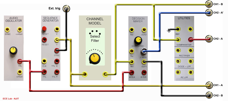
Figure 4: the COMPARATOR and DECISION MAKER as regenerators

The macro CHANNEL MODEL module was introduced in the experiment entitled The noisy channel model (within this Volume). It is used for inserting noise, bandlimiting, and adjusting signal levels. As a reminder the model is reproduced here as Figure 5. To provide an adjustable bandwidth, it uses the TUNEABLE LPF as the bandlimiting module.

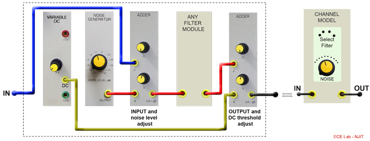
Figure 5: details of the macro CHANNEL MODEL module

Signal Regeneration

First patch up the complete system, according to the block diagram of Figure 3, shown modelled in Figure 4.

Note That:

For selecting the best sampling instant the eye pattern is preferred.
The oscilloscope is triggered externally by the bit clock. To check, visually, that the recovered sequence is error free, you need the snapshot. The oscilloscope is triggered externally by the SYNC pulse of the SEQUENCE GENERATOR.

Ideally, for visual evaluation, the first of these requires a long sequence, and the second a short sequence. For convenience, however, you may find it acceptable to use short sequence for both observations.

T1 Before plugging in the SEQUENCE GENERATOR module select the minimum length sequence with the on-board switch SW2 (both toggles UP).

T2 Model the complete system illustrated in Figure 4, except for the DECISION MAKER. Leave the Z-Mod output from the decision maker un-connected for now.

T3 Set the AUDIO OSCILLATOR to about 2 kHz. This will suit the DECISION MAKER, which has been designed for operation with clock rates of this order.

T4 Ensure the oscilloscope is triggering on the SYNC signal from the SEQUENCE GENERATOR. Check the sequence on CH1-A.

Using the Comparator

T5 Set the TUNEABLE LPF to its widest bandwidth. Check the signal on CH1-B is roughly of the same shape as shown in Figure 1. The COMPARATOR should have no trouble regenerating this sequence.

T6 Check the COMPARATOR output against the original sequence by looking at CH1-A and CH2-A simultaneously. Satisfy yourself that regeneration is acceptable.

T7 Now carry out some observations of the COMPARATOR output as either or both the channel bandwidth is varied and noise is added. Get some appreciation of the imitations of the COMPARATOR as a regenerator.

Signal Levels

No mention was made above about the signal levels at the various interfaces. You should be experienced enough now to realize how important these are. Although this may seem to be a digital-style experiment, most of the modules are processing analog-level signals. So the signal levels at their (yellow) interfaces should be adjusted appropriately. That is, they should be at about the TIMS ANALOG REFERENCE LEVEL, or 4 volt peak-to-peak. Check back that this was achieved.

DC Threshold

You can investigate the purpose of the DC threshold adjustment provided in the CHANNEL MODEL. Slowly reduce the channel output amplitude, whilst monitoring the COMPARATOR output. Eventually, as the signal amplitude is progressively decreased, the COMPARATOR output will be all HI or all LO. Fine adjustment of the DC level from the channel 1 will re-position the sequence with respect to the COMPARATOR reference level (nominally zero, or ground) and allow operation for even smaller input levels.

Using the Decision Maker:

T8 Read about the DECISION MAKER module in the TIMS Advanced Modules User Manual. Before plugging it in, ensure that:

The on-board switch SW2 is switched to ‘INT’

The ‘NRZ-L’ waveform is selected with on-board switch SW1

(upper rear of board). This configures the DECISION MAKER to accept bipolar non-return-to-zero waveforms, as you have from the analog output of the SEQUENCE GENERATOR.

Set the gain ‘g’ of the ADDER to some small, finite value, and use the VARIABLE DC front panel control to adjust the voltage. This allows a finer adjustment.

T9 Change the oscilloscope triggering, and display to an eye pattern.

T10 Patch the DECISION MAKER into the system. Now connect the Z-MOD connection to Channel 2-B. Display Ch. 2-B on the oscilloscope along with the received signals eye diagram on Channel 1-B. The Oscilloscope should display the gating signal for the Decision maker indicating when during the bit period the Decision Maker makes its decision.

T11 Rotate the front panel DECISION POINT control knob of the DECISION MAKER. The comb signal of the Z-Mod output will slide relative to the sys diagram.

Note: Make sure a TTL bit clock is connected to B.CLK in.

T13 Adjust the front panel control of the DECISION MAKER so that the sampling instant is positioned at the best decision point within the bit period; ie, where the vertical eye opening is greatest.

T14 Display the regenerated sequence and compare it with the input sequence. There will, of course, be a time offset between the two, due to the delay introduced by the filter, and the regeneration process itself.

Note that the DECISION MAKER provides a new bit clock, aligned with the regenerated sequence. This is essential for later processing of the regenerated sequence (eg, by the error counter - see later). You will now make some more demanding tests of the DECISION MAKER. Changing from one display to the other involves a little more than changing the connection to the ext trig of the oscilloscope, as generally the sweep speed needs some slight adjustment. Ideally, also, the snapshot needs a short sequence, and the eye a long sequence. But for these tests a short sequence should be acceptable for both. What you will have to do, each time you make a test, is:

Lower the bandwidth a little

Re-position the sampling instant

Check the sequences for equality

You can develop your own visual scheme for comparing sequences.

T15 Now carry out some observations of the DECISION MAKER output, as you did for the COMPARATOR output, as either or both the channel bandwidth is varied and noise is added. Get some idea of the performance of the DECISION MAKER, as compared with that of the simple COMPARATOR, as a regenerator.

Error Counting

During the above observations you may have been saying ‘there must be a better way to judge performance?’ And, of course, there is! A visual check for errors provides a quick method for comparing short sequences, but it is a qualitative check only; something quantitative is then required for serious measurements. More systematic methods are introduced later in this experiment in the section titled entitled BER measurement in the noisy channel

Summing Up

The DECISION MAKER module will be used in many more experiments, so it is important to have a good understanding of its capabilities and limitations.

Tutorial Questions

Q1 Explain why a strobed decision process can be expected to result in a lower incidence of errors, compared to an ungated (instantaneous) comparator.

Q2 Familiarize yourself with the terms ‘timing jitter’ and ‘baseline wander’. Explain, via the eye pattern, how these affect the satisfactory operation of the detection device.

Q3 In this experiment we use a ‘stolen clock’ to generate the strobe clock at the receiver. Refer to your text book and describe the essence of a clock recovery process in a commercial application.

Part II -Bit Error Rate (BER) Measurement in the Noisy Channel

PREPARATION

Overview

This part serves as an introduction to bit error rate (BER) measurement. It models a digital communication system transmitting binary data over a noisy, bandlimited channel. A complete instrumentation setup is included, that allows measurement of BER as a function of signal-to-noise ratio (SNR). Many variations of this system are possible, and the measurement of the performance of each of these can form the subject of separate experiments.

In this first experiment the system is configured in its most elementary form. Other experiments can add different forms of message coding, line coding, different channel characteristics, bit clock regeneration, and so forth.

The Basic System

A simplified block diagram of the basic system is shown in Figure BER-1 below

Figure BER-1: Block diagram of system

The system can be divided into four sections:

The transmitter. At the transmitter is the originating message sequence, from a pseudo random binary sequence (PRBS) generator, driven by a system bit clock.

The channel. The channel has provision for changing its bandlimiting characteristic, and the addition of noise or other sources of interference.

The receiver. The receiver (detector) regenerates the transmitted (message) sequence. It uses a stolen bit clock.

The BER instrumentation. The instrumentation consists of the following elements:

A sequence generator identical to that used at the transmitter. It is clocked by the system bit clock (stolen, in this case). This sequence becomes the reference against which to compare the received sequence.

A means of aligning the instrumentation sequence generator with the received sequence. A sliding window correlator is used. This was introduced in the experiment entitled Detection with the DECISION MAKER in Volume D1.

A means of measuring the errors, after alignment. The error signal comes from an X-OR gate. There is one pulse per error. The counter counts these pulses, over a period set by a gate, which may be left open for a known number of bit clock periods.

A More Detailed Description

Figure 2: block diagram of system in more detail

Figure BER-2: Block diagram of system in more detail

Having examined the overall operation of the basic system, and gained an idea of the purpose of each element, we proceed now to show more of the specifics you will need when modelling with TIMS. So Figure BER 1 has been expanded into Figure BER-2 below. The detector is the DECISION MAKER module, introduced Earlier in this experiment. The LINE-CODE ENCODER and LINE-CODE DECODER modules serve as an interface between the TTL level signals of the transmitter and those of the analog channel. There are a variety of jobs that LINE-CODING and DECODING perform including:

Spectrum shaping and relocation without modulation or filtering. This is important in telephone line applications, for example, where the transfer characteristic has heavy attenuation below 300 Hz.
Bit clock recovery can be simplified.
DC component can be eliminated; this allows AC (capacitor or transformer) coupling between stages (as in telephone lines). Can control baseline wander (baseline wander shifts the position of the signal waveform relative to the detector threshold and leads to severe erosion of noise margin).
Error detection capabilities.
Bandwidth usage; the possibility of transmitting at a higher rate than other schemes over the same bandwidth.

Terminology

Unipolar signaling: where a ‘1’ is represented with a finite voltage V volts, and a ‘0’ with zero voltage. This seems to be a generally agreed-to definition. TTL coding is unipolar with a ‘1’ represented as +5 Volts.
Those who treat polar and bipolar as identical define these as signaling where a ‘1’ is sent as +V, and ‘0’ as -V. They append AMI when referring to three level signals which use +V and -V alternately for a ‘1’, and zero for ‘0’ (an alternative name is pseudoternary). You will see the above usage in the TIMS Advanced Modules User Manual, as well as in this text. However, others make a distinction. Thus:
Polar signaling: where a ‘1’ is represented with a finite voltage +V volts, and a ‘0’ with -V volts.
Bipolar signaling: where a ‘1’ is represented alternately by +V and -V, and a ‘0’ by zero voltage.
The term ‘RZ’ is an abbreviation of ‘return to zero’. This implies that the particular waveform will return to zero for a finite part of each data ‘1’ (typically half the interval). The term ‘NRZ’ is an abbreviation for ‘non-return to zero’, and this waveform will not return to zero during the bit interval representing a data ‘1’.

Figure 2: block diagram of system in more detail. The extra detail in Figure BER-2 includes:

Provision for adding noise to the channel via the adder on the input side of the bandlimiting channel.
Inclusion of an ADDER on the output side of the channel. This restores the polarity change introduced by the input ADDER (for line codes which are polarity sensitive). It also provides an opportunity to fine-trim the DC level to match the threshold of the DECISION MAKER.
Instrumentation for SNR adjustment (not shown) and BER measurement.

Theoretical Predictions

Bit error probability (P_B) is a function of E_n/N_o. For matched filter reception of bipolar baseband signaling it has been shown that: 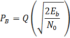...1

The symbols are defined in the Chapter entitled BER macro module .

You will measure not P_B, but BER; and not En/No , but SNR. Figure BER-3 shows theoretical predictions, based on eqn(1) above.

Figure 3 theoretical expectations - BER versus SNR (for bi-polar signaling)

Figure BER-3: Theoretical expectations - BER versus SNR (for bi-polar signaling)

Experiment

Familiarity with the setting up of a transmitter, receiver, and noisy channel, using a stolen clock for bit clock synchronization, and the sliding window correlator for sequence alignment, is assumed. The system under examination, the principle of which is illustrated in block diagram form in Figure 1, is shown modelled by the patching diagram of Figure 4 on the next page. Within that diagram is included the macro CHANNEL MODEL module, and the BER INSTRUMENTATION macro module. The macro CHANNEL MODEL module was introduced in a previous experiment. As a reminder, details of the macro CHANNEL MODEL module are reproduced in Figure BER-4 below.

Figure 4: Details of the macro CHANNEL MODEL module.

Figure BER-4: Details of the macro CHANNEL MODEL module

Remember that, during testing, and afterwards, the oscilloscope triggering comes from:

The SYNC output from the transmitter SEQUENCE GENERATOR for snapshots
The bit clock for eye patterns.

The Error Counting Utilities Module

This is the first time the pulse counting capabilities of the ERROR COUNTING UTILITIES module have been used. A complete description of the characteristics and behavior of the module can be obtained from the TIMS Advanced Modules User Manual. A condensed description of its function is given in the Chapter entitled Digital utility sub-systems, under the two headings Timed Pulse (for the counting function) and Exclusive-OR.

Modelling The Transmission System

The system to be modelled is shown in Figure BER-5. It will be patched up systematically, section by section, according to the scheme detailed below. It has not been cluttered by showing oscilloscope connections. You should set up the SCOPE SELECTOR for maximum usage of the facility for toggling between the A and B options for each channel.

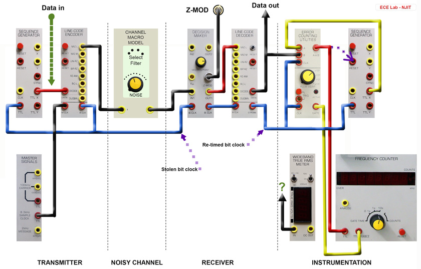
Figure BER-5: The TIMS model of Figure 2

The Transmitter

T1.1 Patch the transmitter according to Figure BER-5, from a SEQUENCE GENERATOR (set to a short sequence - both toggles of SW2, on circuit board, UP), a LINE-CODE ENCODER (using NRZ-L), a LINE-CODE ENCODER (using NRZ-L), and the MASTER SIGNALS module. Note that the LINE-CODE ENCODER accepts the master clock, which is the 8.333 kHz TTL ‘sample clock’ from the MASTER SIGNALS module, and divides it by four to produce the 2.083 kHz system bit clock for the SEQUENCE GENERATOR.

T1.2 Press the reset on the LINE-CODE ENCODER. Check on CH1-A that a short TTL sequence has been generated by the SEQUENCE GENERATOR.

T1.3 Simultaneously with the previous observation on CH1-A, check the NRZ-L output of the LINE-CODE ENCODER on CH2-A. Relative to the TTL on CH1-A it will be delayed half a bit period. This is the signal being transmitted to the channel. Confirm the code format.

T1.4 Switch the output to view some of the other coding schemes. Record the waveforms if some of these for your report.

2.0 The Channel Model

The macro CHANNEL MODEL module is shown modelled in Figure 4.

T2.1 Patch up the channel according to Figure 4 and insert it into the position shown in Figure 5.

T2.2 Set the front panel attenuator of the NOISE GENERATOR to maximum output; but reduce the channel noise to zero by rotating the INPUT ADDER gain control ‘g’ fully anti-clockwise.

T2.3 Adjust the amplitude of the signal into the BASEBAND CHANNEL FILTERS module to near the TIMS ANALOG REFERENCE LEVEL (say, 2 volt peak-to-peak) with the INPUT ADDER gain control ‘G’. This level will need resetting when noise is added.

T2.4 Select channel #3 of the BASEBAND CHANNEL FILTERS module.

T2.5 Set the gain of the DC threshold adjustment path through the OUTPUT ADDER to zero.

T2.6 Adjust the amplitude of the signal out of the CHANNEL MODEL to, say, 2 volt peak-to-peak with the OUTPUT ADDER gain control ‘G’. The gain through the channel is now unity.

T2.7 Confirm that the signal at the OUTPUT ADDER, although of different shape, and further delayed, is clearly related to the input sequence.

When tracing the sequence through the system, notice that there is a polarity inversion introduced by the INPUT ADDER of the channel, and a second inversion introduced by the OUTPUT ADDER.

3.0 The Receiver

The receiver consists of the DECISION MAKER and LINE-CODE DECODER modules.

T3.1 before plugging in the DECISION MAKER:

Switch the on-board switch SW2 to ‘IN’ (DECISION POINT can now be adjusted with the front panel control).

Select the expected line code with the on-board rotary switch SW1 (upper rear of board). For this experiment it is NRZ-L.

T3.2 Patch up the DECISION MAKER, including the Z-MOD output to the oscilloscope.

T3.3 Trigger the oscilloscope from the bit clock, and obtain an eye pattern at the channel output. Adjust the sampling instant, with the DECISION MAKER front panel control, to the center of the eye.

T3.4 Trigger the oscilloscope from the SYNC output of the transmitter SEQUENCE GENERATOR. Check that the reconstructed ‘analog’ output from the DECISION MAKER is a delayed version of, but otherwise the same shape as, that at the channel input.

T3.5 Refer to the DECISION MAKER in the TIMS User Manual for threshold level information. This varies according to the code in use. For the NRZ-L code the threshold is approximately 25 mV. Thus the input signal amplitude must either swamp any possible DC threshold, or, if small, must be adjusted to straddle it. There is provision in the model (the OUTPUT ADDER) for this; it will be checked in the next Section. For now confirm that the output waveform is centered approximately about zero volts.

T3.6 patch up the LINE-CODE DECODER, selecting the NRZ-L output.

T3.7 press the reset on the LINE-CODE DECODER. Check that the TTL output sequence is identical, except for a delay, with that at the transmitter SEQUENCE GENERATOR output. Do not proceed unless these two TTL signals are identical!

4.0 The Bit Error Rate Instrumentation

The transmission system is now fully set up. You will now proceed to verify its overall operation. The BER measurement instrumentation system is used to generate an identical sequence to that transmitted, and aligned with that from the receiver detector. These two sequences will be compared, bit by bit, and any disagreements counted. The count is made over a pre-determined number of bit clock periods, and so the bit error rate (BER) may be calculated. You will record the BER for various levels of noise, and compare with theoretical expectations.

T4.1 Patch up according to Figure 5. Note the instrumentation (receiver) SEQUENCE GENERATOR uses the LINE-CODE DECODER strobe as its bit clock. Trigger the oscilloscope for a snapshot. Check that there is a short sequence coming from the instrumentation SEQUENCE GENERATOR output.

T4.2 See the Appendix to this experiment for a short description of the ERROR COUNTING UTILITIES module, including on-board jumper and switch settings. Plug it in. Check that the line from the X-OR output to the instrumentation SEQUENCE GENERATOR RESET is open.

T4.3 Observe the two inputs to the X-OR gate simultaneously. It is unlikely that they are aligned, but they should be synchronized. Your good work is about to be rewarded with the sight of the two sequences snapping into alignment.

T4.4 Momentarily close the line from the X-OR output to the instrumentation SEQUENCE GENERATOR RESET. Confirm that the two sequences, already synchronized, are now aligned. If you want to see the sliding window correlator at work again, press the reset on the instrumentation SEQUENCE GENERATOR, and alignment will be lost. Realign by repeating the last Task.

T4.5 Set the FREQUENCY COUNTER to its COUNT mode, and patch it into the system, complete with the gate signal from the ERROR COUNTING UTILITIES module.

T4.6 Switch the gate of the ERROR COUNTING UTILITIES, with the PULSE COUNT switch, to be active for 10⁵ bit clock periods. Make a mental calculation to estimate how long that will be!

T4.7 To make an error count: a) reset the FREQUENCY COUNTER. b) start the error count by pressing the TRIG button of the ERROR COUNTING UTILITIES module. The ‘active’ LED on the ERROR COUNTING UTILITIES module will light, and remain alight until 90% of the count is completed, when it will blink before finally extinguishing, indicating the count has concluded. With no noise there should be no errors.

But .....

Warning: Every time a count is initiated one count will be recorded immediately. This is a ‘confidence count’, to reassure you the system is active, especially for those cases when the actual errors are minimal. It does not represent an error, and should always be subtracted from the final count.

Despite the above single confidence-count you may wish to make a further check of the error counting facility, before using noise.

T4.8 I f the ERROR COUNTING UTILITIES GATE is still open press the instrumentation SEQUENCE GENERATOR reset button (else press the TRIG to open the GATE). The sequences should now be out of alignment. The counter will start counting (and continue counting) errors until the GATE shuts. It will record a count of between 2 and 10ⁿ (with the PULSE COUNT switch set to make 10ⁿ counts). You will record a different count each time this is repeated. Why would this be?

Well done ! You have just completed a major setting-up procedure. If it was achieved without any problems you are to be congratulated! Although TIMS itself will behave reliably, it is easy to make patching errors, and their discovery and rectification is all part of the learning process.

You are now almost ready to sit back and let TIMS do the measurements for you.

5.0 Error Counting with Noise

Preparation

T5.1 Increase the message sequence length of both SEQUENCE GENERATOR modules (both toggles of SW2 DOWN). See Tutorial Question Q2.

T5.2 Re-establish sequence alignment by pressing all the reset buttons, in order input to output, then momentarily connect the X-OR output to the instrumentation SEQUENCE GENERATOR RESET input.

Adding Noise - Principle

It is now time to add the noise to the signal. Noise must be introduced before bandlimiting, since the channel bandlimiting filters are required to bandlimit the noise as well. The noise from the NOISE GENERATOR is wideband. Its peak amplitude must not overload an analog module, so its output has been restricted to 4 volt peak-to-peak (the TIMS ANALOG REFERENCE LEVEL). As soon as it is bandlimited, this amplitude is reduced. Amplification cannot be used to bring it up to a convenient level until after bandlimiting. But by this time the signal has been added, so that is not possible. So the only way to obtain a small signal-to-noise ratio (relatively high noise) is to reduce the signal level. This is done with the INPUT ADDER. To set the noise level:

Remove the signal from the channel input

Add as much noise as is available, to implement the worst SNR possible, by maximizing the gain through the INPUT ADDER, and setting the attenuator of the NOISE GENERATOR for maximum noise output. The SNR can later be increased - less noise - with this attenuator.

Measure the noise level into the DECISION MAKER with the WIDEBAND TRUE RMS METER. Then remove the noise, replace the signal, and adjust it to the same level.

Replace the noise. The SNR is 0 dB.

The system is now set up for the worst conditions under which measurements are to be made. From now on the SNR will be improved, in calibrated steps of the NOISE GENERATOR attenuator, and BER measurements recorded. The above steps will now be implemented.

Adding Noise - Practice

T5.3 Patch both the oscilloscope and the WIDEBAND TRUE RMS METER to observe the signal at the output of the channel.

T5.4 Reduce the signal amplitude to zero with the ‘G’ gain control of the INPUT ADDER.

T5.5 Set the attenuator of the NOISE GENERATOR for maximum output. Increase the noise level into the channel, with the INPUT ADDER, to maximum. Record the reading of the rms meter (N volt rms amplitude).

T5.6 Remove the noise by unplugging the patch cord from the INPUT ADDER.

T5.7 Introduce some signal with the ‘G’ control of the channel INPUT ADDER, until the rms meter is reading the same as the previous noise reading. Record this reading (S volt rms amplitude). BER measurement in the noisy channel

T5.8 Replace the noise. Do not disturb the INPUT ADDER gain settings from now on!

T5.9 Check the signal level at the channel output. Use the ‘G’ gain control of the OUTPUT ADDER to raise the input level to the DECISION MAKER to the TIMS ANALOG REFERENCE LEVEL (4 V peak-to-peak is allowable, although there may be insufficient gain in the ADDER).

The SNR is now set up to a reference value s2/n2

and this will be 0 dB. However you may have your own reasons for selecting some other ratio, but it needs to result in many errors. From now on you can only reduce the noise, using the calibrated attenuator of the NOISE GENERATOR. This will increase the SNR, which will in turn reduce the error rate. Warning: if alignment is ever lost, the noise must be removed before attempting re-alignment!

T5.10 set the SNR to, say, 10 dB, and set the decision instant with the aid of an eye pattern.

6.0 DC Offset Adjustment

The effect of any DC threshold of the DECISION MAKER must be offset with DC introduced by the OUTPUT ADDER. Two methods are suggested. 1. after setting up as above, add a small DC to the signal from the channel. If the error count can be reduced then adjust for the smallest count. 2. set the DC output from the channel to +25 mV. This is the threshold level of the DECISION MAKER in NRZ-L mode. Now implement one or the other method of threshold adjustment

Method 1:

T6.1 Set the PULSE COUNT on the DECISION MAKER to 10⁵ and press the TRIG button. Adjust the noise level with the attenuator so that errors are accumulating at about 10 per second (watch the second last digit).

T6.2 Rotate the VARIABLE DC level about 450 anti-clockwise. Advance the ‘g’ control of the OUTPUT ADDER about 200. The error rate should increase.

T6.3 Slowly reduce the DC offset voltage magnitude (rotate the VARIABLE DC control clockwise towards zero). The error rate should slowly reduce, then increase. Return to the lowest rate and stay there. This is an important adjustment. It takes some practice. At all times set the error rate (with the noise source attenuator) so it is about 10 errors per second. Concentrate on the second last, and then the last digit, as the minimum is approached.

Method 2:

T6.4 Remove both inputs from the INPUT ADDER. Using both the VARIABLE DC control and the OUTPUT ADDER ‘g’ control, set the DC level at the input to the DECISION MAKER +25 mV (use the WIDEBAND TRUE RMS METER). Replace the inputs to the INPUT ADDER.

Measuring the BER

Everything is now set up for some serious measurements. It is assumed that:

Both SEQUENCE GENERATORS are set for long sequences (both toggles of the on-board switch SW2 are DOWN).
Line code NRZ-L has been patched (for this experiment) on the LINE-CODE ENCODER and LINE-CODE DECODER.
Line code NRZ-L has been selected with SW1 on the DECISION MAKER board.
All reset button have been pushed (in turn from input to output).
Levels throughout the system have been set correctly (typically with SNR = 0 dB with max noise from the NOISE GENERATOR).
DC threshold at the DECISION MAKER has been accounted for
Signal into the DECISION MAKER is ideally at the TIMS ANALOG REFERENCE LEVEL (but probably considerably lower with the model of Figure 4).
The DECISION POINT of the DECISION MAKER has been set up, using an eye pattern (with ‘moderate’ noise present - say an SNR of 10 dB).
The SEQUENCE GENERATOR at the receiver has been aligned with the incoming sequence (carried out with no noise present - a high SNR).
Conditions for a known (reference) SNR are recorded.
Channel bandwidth is recorded (eg, which filter of the BASEBAND CHANNEL FILTERS module is in use.)

T6.5 Measure BER according to the procedure in Task T4.7. Record the measurement, and the conditions under which it was made. Compare results with counts over short and long periods.

T6.6 Decrease the noise level by one increment of the NOISE GENERATOR front panel attenuator. Go to the previous Task. Loop as many times as appropriate.

T6.7 Plot BER versus SNR. Relate your results to expectations.

Role of the Filter

The characteristics of the filter will influence the result. The theoretical results assume an ‘ideal’ filter. We do not have that.

Conclusion

Future experiments will use this system configuration to measure BER under different conditions - for example, with the addition of error control coding, bit clock regeneration, and so on. It is important, then, that you familiarize yourself with the setting up procedures of the basic system which was the subject of this experiment.

Tutorial Questions

Q1 Once sequence alignment is attained, the sliding window correlator is disabled. Explain why alignment is not lost even if the noise level is raised until the BER increases to unacceptably high levels. Explain why it would lead to incorrect error counts to leave it connected during the counting process.

Q2 Why were you advised to use a long sequence when counting errors?

Q3 Explain the principle of what you were doing when adjusting the DC at the input to the DECISION MAKER.