LAB 2: FM MODULATION, DEMODULATION AND BESSEL ZEROS
ACHIEVEMENTS:
Students demonstrate FM generation using a VCO and confirm selected aspects of the FM spectrum. Demodulation using a zero crossing counter demodulator is demonstrated. The method of Bessel Zeros is used to Calibrate the frequency deviation sensitivity of the VCO based FM transmitter.
PREREQUISITES:
Familiarity with the contents of the chapter entitled Analysis of the FM spectrum. A knowledge of the relationships between the frequency deviation and the spectrum of a FM signal. See Appendix C to this text for Tables of Bessel Coefficients.
PRELAB:
Read the section of the manual titled Analysis of the FM Spectrum.
Familiarize yourself with the special modules by reading their descriptions in the posted module handbooks.
In part three of this lab the FM signal is frequency tripled which also triples the phase deviation or depth of modulation of the FM signal. Assume a VCO sensitivity, S, of S = Δf⁄V = 1⁄3 kHz ⁄ Volt. Use Equation 2-1 below to determine the expected rms reading of a voltmeter attached to the modulating input of the VCO for observation of the first zero of the zeroth order Bessel function using a carrier frequency of fc=11.11 kHz and a message frequency of fm=1KHz.
Extra Modules:
VCO, TWIN PULSE GENERATOR, AUDIO OSCILLATOR, True-RMS VOLTMETER, UTILITIES, 100 kHz CHANNEL FILTERS and FM UTILITIES.
You may want to use a hand held DMM as well.
LAB
Introduction
This experiment is an introduction to FM signals. In the first part a voltage controlled oscillator is explored as a source of FM. The second part introduces the zero crossing detector as an FM Demodulator and the third part examines the VCO sensitivity to a time varying signal.
The VCO - voltage controlled oscillator- is available as a low-cost integrated circuit (IC), and its performance is remarkable. The VCO IC is generally based on a bi-stable 'flip-flop', or 'multi-vibrator' type of circuit. Thus its output waveform is a rectangular wave. However, ICs are available with this converted to a sinusoid. The mean frequency of these oscillators is determined by an RC circuit.
The controllable part of the VCO is its frequency, which may be varied about a mean by an external control voltage. The variation of frequency is remarkably linear, with respect to the control voltage, over a large percentage range of the mean frequency. This then suggests that it would be ideal as an FM generator or communications purposes. Unfortunately such is not the case. The relative instability of the center frequency of these VCOs renders them unacceptable for modern day communication purposes. The uncertainty of the center frequency does not give rise to problems at the receiver, which may be taught to track the drifting. The problem is that spectrum regulatory authorities insist, and with good reason, that communication transmitters maintain their (mean) carrier frequencies within close limits.
It is possible to stabilize the frequency of an oscillator, relative to some fixed reference, with automatic frequency control circuitry. But in the case of a VCO which is being frequency modulated there is a conflict, with the result that the control circuitry is complex, and consequently expensive. For applications where close frequency control is not mandatory, the VCO is used to good effect.
FFT Spectrum
Examination of the spectrum will be carried out by using the Fast Fourier Transform feature of the oscilloscopes. You should be familiar with this feature from using it in the first lab. In the first part of the lab, two spectral properties of an FM signal will be examined: the first zero of the carrier amplitude and the modulation depth leading to equal amplitudes of the carrier and the first side bands.
Special Cases, β= 1.45 and β= 2.405
For β = 1.45 the amplitude of the first pair of sidebands is equal to that of the carrier; and this will be J0(1.45) times the amplitude of the unmodulated carrier (always available as a reference). You should confirm this result from Tables of Bessel functions (see, for example, the Appendix C to this volume). For β = 2.405 the amplitude of the carrier should fall to zero. These are two of the many special cases one can examine to further verify the predictions of theory.
Zero-Crossing demodulator
In part two a zero-crossing detector and a low pass filter will be used to de-modulate the FM signal generated in part one. Figure 1. shows an FM signal and the output from a zero-crossing detector as a function of time.
Figure 1: an FM signal, and a train of zero-crossing pulses
Each pulse in the pulse train is of fixed width, and is located at a zero crossing of the FM signal. This is a pulse-repetition-rate modulated signal. If the pulse train is passed through a low-pass filter, the filter will perform an averaging operation. The rate of change of this average value is related to the message frequency, and the magnitude of the change to the depth of modulation at the generator.
This zero-crossing-counter demodulator will be modelled in the latter part of the experiment.
Bessel Zero Method of Calibration
The third part investigates the deviation calibration of an FM transmitter by observation of the spectrum using the method of 'Bessel zeros'. The outcome of the experiment should be a calibration curve, showing the achieved modulation deviation as expressed by β versus the peak voltage applied to the modulator. The modulation index, β, is given by the following equation
![]() Equation 2-1
Equation 2-1
where Vin is the amplitude of the modulation input signal, S is the sensitivity of the VCO as measured in part 1 and fm is the modulating frequency.
This curve will have already been obtained for DC voltages. Here you will be examining the spectrum, and from this working backwards to determine the phase deviation and ultimately if the VCO sensitivity is the same for DC and for a kHz modulation.
As in part 1, the Voltage Controlled Oscillator is used to generate the FM signal. However, at 1 kHz/Volt sensitivity it is difficult to set the input voltage accurately enough to find the nulls. As a result of reducing the sensitivity in this part, the modulator can't provide enough phase deviation to find more than one or side band zeros. To increase the modulation depth, the output will be converted to its third harmonic increasing the range of phase deviation by a factor of three. We use a frequency multiplier to effect this. Here we call it a deviation multiplier as we are concerned with increasing the phase deviation or modulation depth (β) rather than the carrier frequency. NOTE: the modulation frequency is not multiplied by 3 in this process.
The multiplication is affected by passing the VCO output through a limiter which generates odd harmonics and then passing this signal through a band-pass filter at the third harmonic frequency of the carrier. Both the limiter and the filter are contained in the FM utilities module.
You should make certain that you understand how the signal changes during this process. This is explained in the limiting section of the document 'Analysis of the FM Spectrum'.
Experiment
Part I: VCO Calibration and FM Generation
A suitable set-up for measuring some properties of a VCO is illustrated in Figure 2.
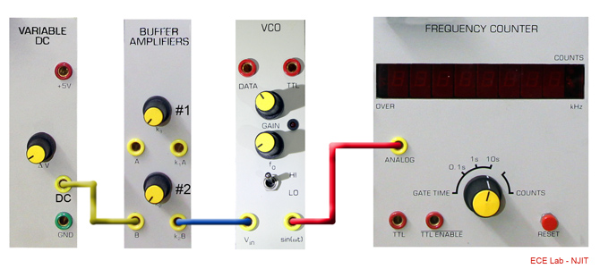
Figure 2: the FM generator
For this experiment you will measure the sensitivity of the frequency of the VCO to an external control voltage, so that the frequency deviation can be set as desired.
The mean frequency of the VCO is set with the front panel control labelled fo. The mean frequency can as well be varied by a DC control voltage connected to the Vin socket. Internally this control voltage can be amplified by an amount determined by the setting of the front panel GAIN control. Thus the frequency sensitivity to the external control voltage is determined by the GAIN setting of the VCO.
A convenient way to set the sensitivity (and thus the GAIN control, which is not calibrated), to a definable value, is described below.
T1 Before plugging in the VCO, set the mode of operation to 'VCO' with the onboard switch SW2. Set the front panel switch to 'LO'. Set the front panel GAIN control fully anti-clockwise.
T2 Patch up the model of Figure 2.
T3 Use the FREQUENCY COUNTER to monitor the VCO frequency. Use the front panel control fo to set the frequency close to 11.11 kHz. This frequency is chosen as its third harmonic is centered in the pass-band of the filter in the FM Utilities module which will be used in part three.
Deviation Sensitivity
T4 Set the VARIABLE DC module output to about 2 volt. Connect this DC voltage, via BUFFER #2, to the Vin socket of the VCO.
T5 With the BUFFER #2 gain control, set the DC at the VCO Vin socket to exactly -1.0 volt. With the VCO GAIN set fully anti-clockwise, this will have no effect on f0.
T6 Adjust the GAIN control of the VCO to give a 1 kHz peak frequency deviation for a modulating signal at Vin of -1 volt. Turn the gain control until the frequency has changed by 1000 Hz. Record the exact values of the input voltage to the VCO and the output frequency change to determine its sensitivity at this gain level.
The gain control setting will now remain unchanged. For this setting you have calibrated the sensitivity, S, of the VCO to 1 kHz/Volt. Do not change the VCO gain control until told to do so near the start of part 3!
Deviation Linearity
The linearity of the modulation characteristic can be measured by continuing the above measurement over a range of input DC voltages. If a curve is plotted of DC volts versus frequency deviation the linear region can be easily identified.
A second, dynamic, method would be to use a demodulator, using an audio frequency message.
T7 Take a range of readings of frequency versus DC voltage at Vin of the VCO, sufficient to reveal the onset of non-linearity of the characteristic. This is best done by producing a plot as the readings are taken. Report the approximate linear range of the VCO.
The FM Spectrum
So far you have a theoretical knowledge of the spectrum of the signal from the VCO, but have made no measurement to confirm this.
The VARIABLE DC voltage, with a moderate setting of the VCO GAIN control, has been used as a fine tuning control. Now the variable DC will be replaced by a sinusoidal modulation to generate the FM signals. Remember that one is generally not interested in absolute amplitudes - what is sought are relative amplitudes of spectral components. Keep the VCO gain control where you set it in the earlier steps so that the sensitivity, S, remains at approximately 1kHz/volt.
Two such spectra will now be observed.
- The first Bessel zero of the carrier term will be set up.
- The amplitude of the carrier will be made equal to that of each of the first pair of sidebands.
T9 Observe the signal from the VCO on the oscilloscope and display both the signal and the FFT spectrum on the screen at the same time. Record this picture for your report.
T10 Turn the modulating signal down to zero by adjusting the buffer amplifier and observe the carrier component. Set the vertical scale of the spectrum so that it covers most of the screen. Record the amplitude of the carrier in dB.
Equal Carrier and First Sidebands
T11 Adjust the BUFFER amplifier until the first sidebands appear in the spectrum. Continue increasing the modulating signal until the first sidebands are the same height as the carrier frequency component in the spectrum. This should correspond to β = 1.44. Measure the rms value of the modulating voltage at the VCO input. Record the amplitude of the sidebands in dB. Record this image, showing the carrier and first sidebands having the same amplitude in the FM modulator output spectrum.
T12 Adjust the BUFFER amplifier, increasing the modulating signal, to minimize the carrier amplitude in the spectrum. This corresponds to the first time J0(β) = 0, which occurs for β = 1.44. Record the image showing the nulled carrier frequency signal. Measure the modulating signal rms voltage at the input to the VCO.
T13 Find one of the adjacent sidebands. Its amplitude should be J1(β) times the amplitude of the unmodulated carrier (measured previously). Since J1(2.45) ≅ 0.5 then each of the first pair of sideband should be of amplitude half that of the unmodulated carrier 9 or about 3 dB down from the original carrier peak). Check this and record their relative amplitudes.
Calculate the values of β for steps T13 and T12 and compare with the theoretical values in your report.
There are many more special cases, of a similar nature, which you could investigate. In the third part of this lab you will measure some of the other Bessel zeros.
You will now use this generator to provide an input to a demodulator.
Part 2: FM Demodulation
A simple FM demodulator, if it reproduces the message without distortion, will provide further confirmation that the VCO output is indeed an FM signal. A scheme for achieving this result was introduced earlier - the zero-crossing counter demodulator - and is shown modelled in figure 3.
The zero Crossing Counter
A simple yet effective FM demodulator is one which takes a time average of the zero crossings of the FM signal. Figure 1 suggests the principle.
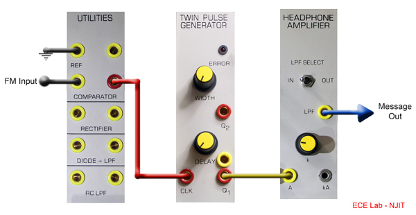
figure 3: an FM demodulator using a zero-crossing demodulator
The TWIN PULSE GENERATOR is required to produce a pulse at each positive going zero crossing of the FM signal. To achieve this, the FM signal is converted to a TTL signal by the COMPARATOR, and this drives the TWIN PULSE GENERATOR.
Note: the input signal to the HEADPHONE AMPLIFIER filter is at TTL level. It is TIMS practice, in order to avoid overload, not to connect a TTL signal to an analog input. Check for overload. If you prefer you can use the yellow analog output from the TWIN PULSE GENERATOR. This is an AC coupled version of the TTL signal.
T14 Before plugging in the TWIN PULSE GENERATOR set the on-board MODE switch SW1 to SINGLE. Patch up the demodulator of figure 3.
T15 Set the frequency deviation of the FM generator to zero, and connect the VCO output to the demodulator input.
T16 Using the WIDTH control of the TWIN PULSE GENERATOR adjust the output pulses to their maximum width.
T17 Observe the demodulator output. If you have chosen to take the TTL output from the TWIN PULSE GENERATOR there should be a DC voltage present. Why? Notice that it is proportional to the width of the pulses into the LPF of the HEADPHONE AMPLIFIER.
T18 Introduce some modulation at the VCO with the BUFFER amplifier gain control. Observe the demodulated output from the LPF of the HEADPHONE AMPLIFIER using the oscilloscope. Measure its frequency (and compare with the message source at the transmitter).
T19 Show (TAKE DATA) that the amplitude of the message output from the demodulator:
- varies with the message amplitude into the VCO. Is this a linear variation?
- varies with the pulse width from the TWIN PULSE GENERATOR. Is this a linear variation?
- is constant with the frequency of the message to the VCO. Does this confirm the VCO is producing FM, and not PM?
T20 Increase the message amplitude into the VCO until distortion is observed at the receiver output. Can you identify the source of this distortion? Record the amplitude of the message at the VCO. You may need to increase the GAIN of the VCO.
Part 3: Bessel Zero method of Sensitivity Measurement
Finding the zeros requires balancing having enough sensitivity in the VCO to allow modulation adjustment to find the zeros accurately while having enough dynamic range of this adjustment to see several zeros. We have several controls on the sensitivity. The gain on the VCO should not be used for this as the point of finding the zeros is to calibrate the gain which will be difficult if you keep changing it. The two other controls are the frequency of the modulation and the amplitude of the modulating signal, as β = (SVampl ) ⁄ fm
Locate the Carrier
T21 With β set to zero, locate the unmodulated carrier with the FFT Function on the oscilloscope.
Spectral amplitudes are typically quoted with respect to the amplitude of the unmodulated carrier. Thus it is convenient to set this component to full scale on the measuring equipment. Do your best to accomplish this.
T22 Check that there are no other components of significance within 10 kHz of the carrier.
figure 4: Bessel function plots
The Method of Bessel Zeros
This is a very precise method of obtaining points on the calibration curve. Not only is an absolute amplitude reading not required, but there is only a single measurement to make - and this is a null measurement. There is no need for a calibrated instrument.
Note, from figure 4, that the Bessel functions are oscillatory (but not, incidentally, periodic). In fact they are damped oscillatory, which means that successive maxima are monotonically decreasing. But for the moment the important property is that they are oscillatory about zero amplitude, which means that there are values of their argument for which they become zero. There are precise, and multiple values, of β, for which the amplitude of a particular spectral component of an angle modulated signal falls to zero.
If you can find when the amplitude of a particular spectral component falls to zero, you have a precise measure of β, and a point on the calibration curve.
Looking for a Bessel Zero
Using the FFT
Table 1 below shows some particular Bessel zeros which you can use experimentally. These can be checked by reference to the curves of figure 4.
Table 1, zeros of Bessel functions.
| Modulation frequency, fm = | |||
| Bessel Zero | β | Vrms | (SVampl ) ⁄ fm |
| J0(β)=0 (1st 0) | 2.41 | ||
| J1(β)=0 (1st 0) | 3.83 | ||
| J2(β)=0 | 5.13 | ||
| J3(β)=0 | 6.38 | ||
| J0(β)=0 (2nd 0) | 5.52 | ||
| J1(β)=0 (2nd 0) | 7.02 | ||
| J4(β)=0 | 7.59 | ||
Each Bessel zero will give a point on the calibration curve.
Note that it is necessary to keep track of which zero one is seeking. This is relatively simple when finding the first or second, but care is needed with the higher zeros.
T23 Choose the minimum modulation frequency that allows sufficient sensitivity that allows you to find the zeros, and then adjust the buffer amplifier gain up and down to control Vampl. Record the frequency you choose and keep it constant for this part of the lab. For each zero that you find measure Vrms with either a DMM or the rms voltmeter module. To complete the chart you will need to use Vrms to obtain the signal amplitude, Vampl. Ultimately you will have a chart of β vs. Vampl ⁄ fm. Make a plot of this and find the best fit slope. Record the slope and the uncertainty of it. Note if you see any curvature indicating the VCO is becoming non-linear.
T24 Whilst monitoring the amplitude of the component at carrier frequency, increase the phase deviation control on the VCO from zero until the amplitude is reduced to zero. Record the value of the rms voltage at the input to the VCO.
T25 As for the previous task, locate either of the first pair of side frequencies (33.33 kHz ± message frequency). Increase the phase deviation by increasing the buffer amplifier gain until the amplitude of the chosen component is reduced to zero. Measure and record the rms modulating voltage at the input to the VCO.
T26 Continue as in the previous two steps to find as many the zeros of the carrier and sidebands as you can recording the rms voltage modulating the VCO for each. Determine the sensitivity to the modulating signal amplitude for all zeros you can find .
T27 For an additional point you can look for the first point where the carrier and first side lobes are of equal magnitude. This was observed earlier with 500 Hz modulation and occurs for β = 1.44. There are other values of β when other combinations of sidelobes have equal height and these can be explored if you have time to gain additional data points.
Note that finding this point did not involve the measurement of absolute amplitude, but rather the matching of two amplitudes to equality. So the amplitude sensitivity of the FFT need not be calibrated.
This amplitude matching method can be applied to determine other values of β From the curves of Figure 4 one could suggest the following values for β. You can come back and try to measure some of these after completing the rest of the lab - if you have time Note that the method did not involve the measurement of absolute amplitude, but rather the matching of two amplitudes to equality. So the amplitude sensitivity of the FFT need not be calibrated. This amplitude matching method can be applied to determine other values of β. From the curves of Figure 4 one could suggest the following values for β3. You can come back and try to measure some of these after completing the rest of the lab - if you have time.
Table 2: Equal amplitude side frequency pairs
| β3 | Frequency components that have equal amplitude |
| 1.85 | Carrier and second |
| 2.6 | First and second |
| 3.8 | Carrier and second |
Report Questions
Q1 Name some applications where moderate carrier instability of an FM system is acceptable.
Q2 Capture the amplitude/frequency spectrum of the signal generated in task T14.
Q3 How would you define the bandwidth of the signal you generated in Task T14?
Q4 What will the FREQUENCY COUNTER indicate when connected to the FM signal from the VCO? Discuss possibilities.
Q5 Derive an expression for the sensitivity of the demodulator of Figure 3, and compare with measurements.
Sensitivity = (Output message amplitude ⁄ Input FM frequency
deviation)
Conclusions
There are many other observations you could make.
- Have you checked (by calculation) the bandwidth of the FM signal under all conditions? Could it ever extend 'below DC' and cause wrap-around (foldback) problems?
- Do you think there is any conflict with the nearness of the message frequency to the carrier frequency? Why not increase the carrier frequency to the limit of the VCO on the 'LO' range - about 15 kHz.
- Why not avoid possible problems caused by the relatively large ratio Γ/ω and change to the 100 kHz region?