LAB 1: AMPLITUDE MODULATION
ACHIEVEMENTS:
Modeling of an amplitude modulated (AM) signal; method of setting and measuring the depth of modulation; waveforms and spectra; trapezoidal display.
PREREQUISITES:
A knowledge of DSBSC generation. Thus reviewing of the experiment entitled DSBSC generation would be an advantage.
PRELAB:
In this lab you will begin to look at the frequency power spectrum of signals. This is traditionally done with a Spectrum Analyzer however we will use the FFT capability of our oscilloscopes here. Read about spectrum analyzers. Read about using the FFT on the Tektronix DPO 2000 series oscilloscopes manual.
Understand the differences between swept frequency, FFT, and real-time spectrum Analyzers, as well as the term resolution bandwidth.
An important characteristic of Spectrum analyzers is the noise floor or signal sensitivity. For an FFT based analyzer this is related to the number of bits per sample for the A/D converter. A modern spectrum analyzer can detect signals below -100 dbm. The noise floor or lower limit for our oscilloscope FFTs is closer to -60 dbm. We can use this feature since it won't be a limit for us in this experiment.
Please review the FFT description in the manual for the Tektronix 2000 series scopes on the lab web site under useful links. The FFT is calculated from 5,000 points (typical) of the source waveform. When the input area contains more than 5,000 points, the area is reduced in resolution . The sampling frequency is therefore determined by the length of the waveform sampled. The width of the waveform used for the FFT can be displayed on the screen and is slightly less than the full screen display. Thus the sampling frequency is determined by the horizontal scale setting. For the FFT process, the horizontal scale determines the FFT bandwidth via the sampling frequency and the resolution bandwidth via the length of the signal that is sampled.
Question for Pre-lab: You will be looking at a carrier near 100 kHz that is modulated with close to 1 kHz signal so you will want to be able to see signals separated by 1 kHz at minimum. Determine the screen width in time that provides 1 kHz frequency spacing in the Discrete Fourier Transform. How many cycles of the 100 kHz carrier will be on the screen given the screen width needed?
Please make certain that you also read about the various windowing techniques: Rectangular, Hamming, Hanning and Blackman-Harris. A brief description is in the Tek manual. This will allow you to choose the best one for your lab use.
PREPARATION
In the early days of wireless, communication was carried out by telegraphy, the radiated signal being an interrupted radio wave. Later, the amplitude of this wave was varied in sympathy with (modulated by) a speech message (rather than on/off by a telegraph key), and the message was recovered from the envelope of the received signal. The radio wave was called a 'carrier', since it was seen to carry the speech information with it. The process and the signal were called amplitude modulation, or 'AM' for short.
In the context of radio communication, near the end of the 2Oth century, few modulated signals contain a significant component at 'carrier' frequency. However, despite the fact that a carrier is not radiated. the need for such a signal at the transmitter (where the modulated signal is generated), and also at the receiver, remains fundamental to the modulation and demodulation process respectively. The use of the term 'carrier' to describe this signal has continued to the present day.
As distinct from radio communications, present day radio broadcasting transmissions do have a carrier. By transmitting this carrier the design of the demodulator, at the receiver, is greatly simplified, and this allows significant cost savings.
The most common method of AM generation uses a 'class C modulated amplifier'; such an amplifier is not available in the BASIC TIMS set of modules. It is well documented in text books. This is a 'high level' method of generation, in that the AM signal is generated at a power level ready for radiation. It is still in use in broadcasting stations around the world, ranging in powers from a few tens of watts to many megawatts.
Unfortunately, text books which describe the operation of the class C modulated amplifier tend to associate properties of this particular method of generation with those of AM, and AM generators, in general. This gives rise to many misconceptions. The worst of these is the belief that it is impossible to generate an AM signal with a depth of modulation exceeding 100% without giving rise to serious RF distortion.
You will see in this experiment, and in others to follow, that there is no problem in generating an AM signal with a depth of modulation exceeding 100%, and without any RF distortion whatsoever.
But we are getting ahead of ourselves, as we have not yet even defined what AM is!
Theory
The amplitude modulated signal is defined as:
| AM = E (1 + m·cosμt ) cosωt | ( 1 ) |
| = A (1 + m·cosμt) B cosωt | ( 2 ) |
| = [ low frequency term a(t) ] x [ high frequency term c(t) ] | ( 3 ) |
Here:
'E' is the AM signal amplitude from eqn. ( 1 ). For modeling convenience eqn. ( 1 ) has been written into two parts in eqn. ( 2 ), where (A·B) = E.
'm' is a constant, which, as you will soon see, defines the 'depth of modulation'. Typically m < 1. Depth of modulation, expressed as a percentage, is 100.m. There is no inherent restriction upon the size of 'm' in eqn. (1). This point will be discussed later .
'μ' and 'ω' are angular frequencies in rad/s, where μ/(2·π) is a low, or message frequency, say in the range 300 Hz to 3000 Hz; and ω/(2.π) is a radio, or relatively high, 'carrier' frequency. In TIMS the carrier frequency is generally 100 kHz.
Notice that the term a(t) in eqn. (3) contains both a DC component and an AC component. As will be seen, it is the DC component which gives rise to the term at ω - the 'carrier' - in the AM signal. The AC term 'm.cosμt' is generally thought of as the message, and is sometimes written as m(t). But strictly speaking, to be compatible with other mathematical derivations. the whole of the low frequency term a ( t ) should be considered the message.
Thus:
Figure 1 below illustrates what the oscilloscope will show if displaying the AM signal.
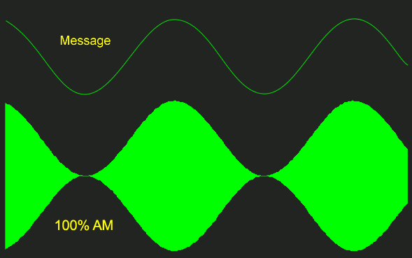
Figure 1 -AM, with m = 1, as seen on the oscilloscope
A block diagram representation of eq. ( 2 ) is shown in Figure 2 below.
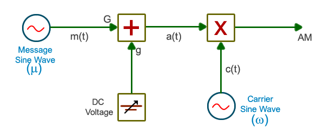
Figure 2: generation of equation 2
For the first part of the experiment you will model eq. (2) by the arrangement of Figure 2. The depth of modulation will be set to exactly 100% (m = 1). You will gain an appreciation of the meaning of 'depth of modulation' , and you will learn how to set other values of 'm " including cases where m > 1.
The signals in eq. (2) are expressed as voltages in the time domain. You will model them in two parts, as written in eq. (3).
Depth of Modulation
100% amplitude modulation is defined as the condition when m = 1. Just what this means will soon become apparent. It requires that the amplitude of the DC (= A) part of a ( t ) is equal to the amplitude of the AC part (= A.m). This means that their ratio is unity at the output of the ADDER, which forces 'm' to a magnitude of exactly unity.
By aiming for a ratio of unity it is thus not necessary to know the absolute magnitude of A at all
Measurement of "m'
The magnitude of 'm' can be measured directly from the AM display itself.
Thus
(5)
where p and Q are as defined in Figure 3.
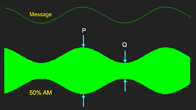
Figure 3: the oscilloscope display for the case m = 0.5
Spectrum
Analysis shows that the sidebands of the AM, when derived from a message of frequency μ rad/s, are located either side of the carrier frequency, spaced from it by μ rad/s.
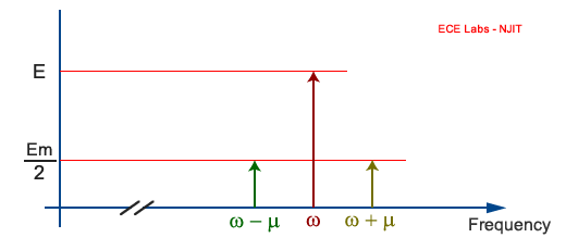
Figure 4: AM spectrum
You can see this by expanding eq. (2). The spectrum of an AM signal is illustrated in Figure 4 (for the case m = 0.75). The spectrum of the DSBSC alone was confirmed in the experiment entitled DSBSC generation. You can repeat this measurement for the AM signal.
As the analysis predicts, even when m > 1, there is no widening of the spectrum.
This assumes linear operation: that is, that there is no hardware overload.
Other message shapes.
Provided m ≤ 1 the envelope of the AM will always be a faithful copy of the message. For the generation method of Figure 2 the requirement is that:
The peak amplitude of the AC component must not exceed the magnitude of the DC,
measured at the ADDER output
As an example of an AM signal derived from speech. Figure 5 shows a snap-shot of an AM signal, and separately the speech signal.
There are no amplitude scales shown, but you should be able to deduce the depth of modulation (the peak depth) by inspection.
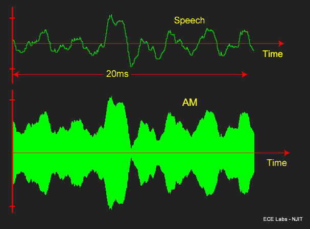
Figure 5: AM derived from speech.
Other Generation Methods
There are many methods of generating AM, and this experiment explores only one of them. Another method, which introduces more variables into the model, is explored in the experiment entitled .Amplitude modulation -method 2, to be found in volume A2- Further & Advanced, Analog Experiments.
It is strongly suggested that you examine your text book for other methods.
Practical circuitry is more likely to use a modulator, rather than the more idealized multiplier. These two terms are introduced in the Chapter of this Volume entitled Introduction to modeling with TIMS, in the section entitled multipliers and modulators.
EXPERIMENT
Aligning the Model
The low frequency term a ( t )
To generate a voltage defined by eq. (2) you need first to generate the term a ( t ).
a ( t ) = A.(1 + m·cosμt) ( 6 )
Note that this is the addition of two parts, a DC term and an AC term. Each part may be of any convenient amplitude at the input to an ADDER.
The DC term comes from the VARIABLE DC module, and will be adjusted to the amplitude 'A' at the output of the ADDER.
The AC term m ( t ) will come from an AUDIO OSCILLATOR, and will be adjusted to the amplitude 'A·m' at the output of the ADDER.
The carrier supply c(t)
The 100 kHz carrier c(t) comes from the MASTER SIGNALS module
c(t) = B.cosωt ( 7 )
The block diagram of Figure 2, which models the AM equation, is shown modeled by TIMS in Figure 6 below.
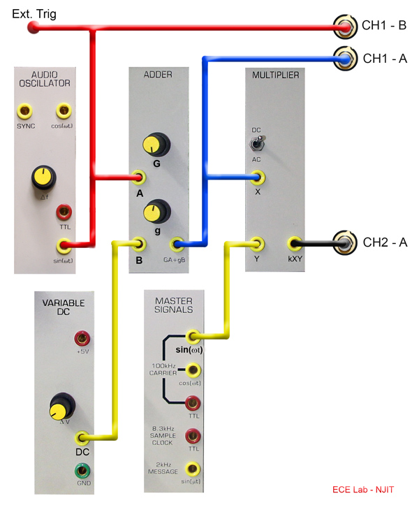
Figure 6: the TIMS model of the block diagram of Figure 2.
To build the model
T1 First patch up according to Figure 6, but omit the input X and Y connections to the MULTIPLIER. Connect to the two oscilloscope channels using the SCOPE SELECTOR, as shown.
T2 Use the FREQUENCY COUNTER to set the AUDIO OSCILLATOR to about 1 kHz.
T3 Switch the SCOPE SELECTOR to CH1-B, and look at the message from the AUDIO OSCILLATOR. Adjust the oscilloscope to display two or three periods of the sine wave in the top half of the screen.
Now start adjustments by setting up a ( t ), as defined by eqn. (4), and with m = 1
T4 Turn both g and G fully anti-clockwise. This removes both the DC and the AC parts of the message from the output of the ADDER.
T5 Switch the scope selector to CH1-A. This is the ADDER output. Switch the oscilloscope amplifier to respond to DC if not already so set, and the sensitivity to about 0.5 volt/cm.
T6 Set gain on ADDER to set VDC
VDC = +1Volt
T7 Now set amplitude of AC signal also to 1 Volt
T8 Connect the output of the ADDER to input X of the MULTIPLIER. Make Sure the MULTIPLIER is switched to accept DC.
Now prepare the carrier signal:
c ( t ) = B.cosωt ( 10 )
T9 Connect a 100 kHz analog signal from the MASTER SIGNALS module to input Y of the MULTIPLIER
T10 Connect the output of the MULTIPLIER to the CH2-A of the SCOPE SELECTOR. Adjust the oscilloscope to display the signal conveniently on the screen.
Since each of the previous steps has been completed successfully, then at the MULTIPLIER output will be the 100% modulated AM signal. It will be displayed on CH2-A. It will look like Figure 1.
Notice the systematic manner in which the required outcome was achieved. Failure to achieve the last step could only indicate a faulty MULTIPLIER?
Agreement with theory
It is now possible to check some theory.
T11 Display the FFT of the waveform on the screen. Vary the time base and determine how it affects the widths of the signal peaks in the FFT, this determines the minimum resolution bandwidth. Using the FFT measure the ratio of power in the carrier to the side lobe(s). In your lab write up compare this with what is expected for a modulation depth of m = 1.
T12 Measure the peak-to-peak amplitude of the AM signal, with m = 1, and confirm that this magnitude is as predicted, knowing the signal levels into the MULTIPLIER, and its 'k' factor.
The significance of 'm'
First note that the shape of the outline, or envelope. of the AM waveform (lower trace), is exactly that of the message waveform (upper trace). As mentioned earlier, the message includes a DC component, although this is often ignored or forgotten when making these comparisons.
You can shift the upper trace down so that it matches the envelope of the AM signal on the other trace. Now examine the effect of varying the magnitude of the parameter 'm'. This is done by varying the message amplitude with the ADDER gain control G.
-
for all values of 'm' less than that already set (m = 1), the envelope of the AM is the same shape as that of the message.
-
for values of m > 1 the envelope is NOT a copy of the message shape.
It is important to note that, for the condition m > 1:
-
it should not be considered that there is envelope distortion, since the resulting shape, whilst not that of the message, is the shape the theory predicts.
-
there need be no AM signal distortion for this method of generation. Distortion of the AM signal itself, if present, will be due to amplitude overload of the hardware. But overload should not occur, with the levels previously recommended, for moderate values of m > 1.
T13 Vary the ADDER gain G, and thus 'm' and confirm that the envelope of the AM behaves as expected, including for values of m > 1. Note both the time-base signal and the FFT on the oscilloscope. Save them for your report for m = .75, m = 1, and m = 1.5 if possible.
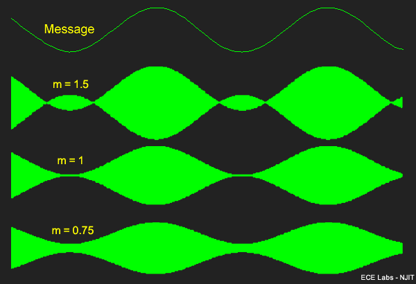
Figure 7: the AM envelope for m < 1 and m > 1.
TUTORIAL QUESTIONS
Q1 There is no difficulty in relating the formula of eqn. (5) to the waveforms of Figure 7 for values of 'm' less than unity. But the formula is also valid for m > 1, provided the magnitudes P and Q are interpreted correctly. By varying 'm' and watching the waveform, can you see how P and Q are defined for m > 1?
Q2 Derive eqn.(5), which relates the magnitude of the parameter 'm' to the peak-to-peak and trough-to-trough amplitudes of the AM signal.
Q3 If the AC/DC switch on the MULTIPLIER front panel is switched to AC what will the output of the model of Figure 6 become?
Q4 An AM signal, depth of modulation 100%.from a single tone message, has a peak-to-peak amplitude of 4 volts. What would an RMS voltmeter read if connected to this signal ? You can check your answer if you have a WIDEBAND TRUE RMS METER module.
Q5 In Task T6, when modeling AM, what difference would there have been to the AM from the MULTIPLIER if the opposite polarity (+ ve) had been taken from the VARIABLE DC module?