Lab 5: 16QAM Modulation
Objective
In this lab, you will observe the 16 QAM modulation and demodulation building Simulink simulation. Then, the second stage will be the implementation of 16 QAM using USRP Hardware.
1. Theoretical Background
Quadrature Amplitude Modulation (QAM) conveys two bit streams by changing the amplitude of two carrier waves that have the same frequency and a 90° shift. The most common type of QAM modulation is rectangular QAM, were the constellation points are arranged in a square grid. Depending on the desired number of bits per symbol (4, 5, 6 …), we have 16QAM, 32QAM, 64 QAM, etc.…
The constellation for 16 QAM is shown in Figure 1
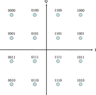
As in QPSK, there are two ways (codes) to map the symbols to the constellation points: Binary code and Gray code. In Gray code, two adjacent symbols differ in one bit, while in Binary code, two adjacent symbols may differ in 2 bits. Therefore, Gray code is preferable over Binary code, since if a receiver maps a symbol to one of its adjacent symbols (due to noise or errors), it will lead to 1 wrong bit instead of 2.
The demodulator maps the received signal (possibly distorted due to noise in the channel) back to bit streams.
For 16 QAM, the Bit Error Rate (BER) is the same as BPSK.
$$ BER=\frac{3}{4} Q\bigg(\sqrt{\frac{4E_b}{N_0}}\bigg) $$Since in QAM modulation two carriers are used, the Symbol Error Rate per carrier is given by:
$$P_{sc}= \frac{6}{4} \: Q\bigg(\sqrt{\frac{E_s}{5N_0}}\bigg) $$And the total Symbol Error Rate is given by:
$$P_s=1- (1- P_sc)^2$$Where $N_0/2$ is the noise power spectral density, and $Q (.)$ is the $Q$ function of the Gaussian distribution.
2. Prelab
- Draw the constellation diagram for 16 QAM. Which bits does each point represent?
- What is the difference between Binary code and Gray code? Which one is better?
- What is the trade-off of using 16 QAM over BPSK?
3. Building Simulink Model of 16 QAM Modulator and Demodulator
- Standard 16 QAM Simulation
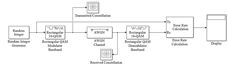
- Build the Simulink model shown in Figure 1.
- Double-click on the Random Integer Generator and adjust the set size to a proper value (Remember that the input to the 16 QAM modulator should be from the set {0, 1, 2, …, 15}).
- In the Random Integer Generator block, set the Sample Time to 1e-6 (i.e. 1 µs) and the Samples per frame parameter to 1024.
- In the AWGN block, set the Symbol period parameter to 1e-6 (i.e. 1 µs) and the Number of bits per symbol parameter to 4 (since 16 QAM uses 4 bits per symbol).
- For the Error Rate Calculation block, set the Output data field to “port” so you can connect the Display block.
- The Display Block will show you three values. The first value is the BER, the second value is the number of incorrect bits, and the third value is the total number of bits received.
- Set the simulation time to 10 seconds.
- In both 16 QAM Modulator and Demodulator blocks, set the Constellation ordering to Gray, set the Normalization method to Peak Power, and set the value of the Peak power to 1 Watt.
- In this experiment, you will adjust the value of the E_b/N_0 in the AWGN block, starting from 3, incrementing by 1 every step, and ending at 15, and observe the error rate displayed in the Display block. Make a table recording the value of E_b/N_0 and the corresponding BER.
- Plot BER vs. E_b/N_0 and compare with the theoretical values. Comment on the results.
- Repeat for different values of the Peak power and plot the results.
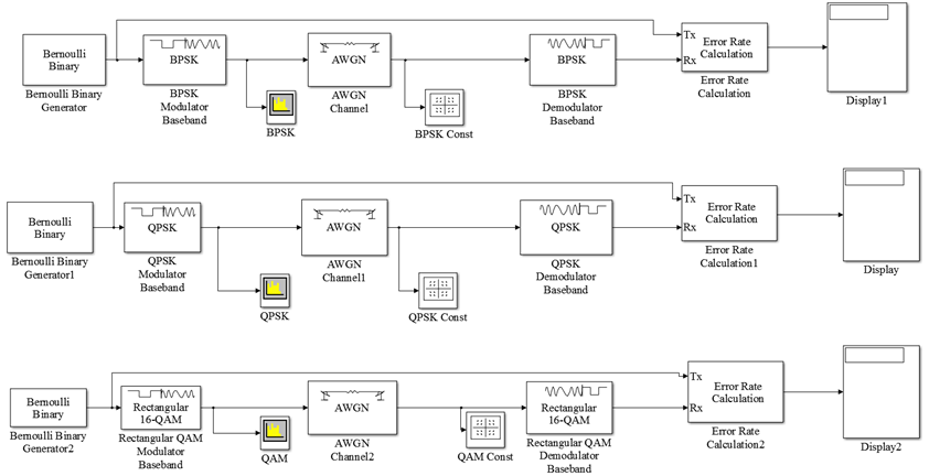
- Comparing 16 QAM, QPSK, and BPSK
- Build the Simulink model shown in Figure 2.
- Double click on the Bernoulli generator for the BPSK part. Set the sample time to 1e-6 and the Samples per frame to 1024.
- Double click on the Bernoulli generator for the QPSK part. Set the sample time to 0.5e-6 and the Samples per frame to 1024.
- Double click on the Bernoulli generator for the 16 QAM part. Set the sample time to 0.25e-6 and the Samples per frame to 1024.
- For the 16 QAM Modulator and Demodulator blocks, use Gray Constellation ordering, set the Normalization method to Peak Power, and set the Peak Power value to 1 Watt.
- Choose the same value of SNR for both AWGN blocks
- Set the simulation time to 10 seconds.
- Run the simulation and observe the bit error rate and the number of transmitted samples from the Display block for both schemes, and observe the used bandwidth for both schemes from the spectrum analyzer block. Explain your observations.
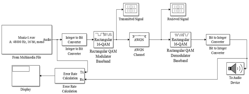
- A Music File Transmission with 16 QAM
- The music file that you will use (named Music-1.wav) is located on the Desktop.
- The music file length is 62 second, so set the Simulation Time to 62 seconds.
- In both Integer to Bit Converter and Bit to Integer Converter blocks, set the Number of bits per integer to 16 (this is related to the music file and not the modulation scheme).
- In both Modulator and Demodulator blocks, use Gray Constellation ordering, set the Normalization method to Peak Power, and set the Peak Power value to 1 Watt.
- In this experiment, you will adjust the value of SNR in the AWGN block and observe the quality of the music. Choose at least three values of SNR (high, mid, low) and comment on the quality of the music.
- Repeat for different normalization methods in the modulator and demodulator blocks.
The Simulink model of 16 QAM modulator and demodulator is shown below
In this experiment, you will learn about the trade-off of using 16 QAM, QPSK, and BPSK.
The following model will be used to simulate a music file transmission using 16 QAM modulation with AWGN channel. You will observe both constellations in the transmitter and the receiver sides and the Bit Error Rate.
4. Simulating Real 16 QAM Transmission
In real transmissions, the transmitted signal may suffer from different types of distortions such as phase errors, amplitude errors, frequency errors, and time jitter. Note that for the previous modulation schemes (BPSK and QPSK) amplitude errors do not make much difference since the information is contained in the phase. However, for 16 QAM, since it is both phase and amplitude modulations, it is sensitive to amplitude errors and DC offset. In this part, you will simulate the effect of these distortions on the transmitted signal and how to correct them.
In this part, you will simulate the effect of these distortions on the transmitted signal and how to correct them.
- Load the file named QAM_param.mat into the workspace by double clicking it.
- Open the file named QAM.slx. This file contains a simulated QAM communication system. The system is shown in Figure 4.
- The Transmitter consists of a Bit generation block and a modulator block.
- The channel adds artificial distortions (frequency, phase, DC level, and delay). Double click on the channel subsystem and examine the components inside.
- The receiver consists of multiple subsystems in order to correct for the distortions added through the channel.
- Open the Frame Synchronization and Decoding subsystem (the last block in the receiver). There you will find a block to calculate BER.
- Run the simulations and observe the BER.
- Observe the constellation points after each stage and take a snapshot to include it in your report. Comment on the effect of each distortion.
