Lab 3- Introduction to Digital Communications-BPSK Modulation

1. Theoretical Background

In the first two experiments, you had experimented the analog modulation techniques AM and FM respectively. Now, the next step is one of the linear modulation technique in digital communications, namely, Binary Phase Shift Keying (BPSK). As known that digital communications are very wide, and you have already taken ECE481. Therefore, we will not include every topic analyzed in digital communications. However, we believe that the overview sections are necessarily be prepared to prevent any gap in your mind. If any point is not clear, please see the course instructor.

Fundamentals of Digital Communications (Overview)

The system model for a digital communication system is given in the following figure;

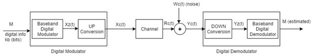
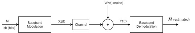
Digital communication has a modulator and demodulator in the same way as in analog communication. The modulator produces an analog signal that is based on the digital data to be transmitted. This analog signal is transmitted over a channel, a cable, or radio waves [1] (in our case, using SDR). The demodulator receives the transmitted signal and constructs an estimate of these digital data.

The digital information M consists of k_b bits. Therefore, it has 2^(k_b ) different and possible messages, and each with different probability such as

For instance,

It does not necessarily to have all probabilities are equal, however we can say that

$k_b=2 →π_0+π_1+π_2+π_3=1$ Thus, the total probability is always equivalent to 1.

Ideally, we want to design a digital modulator and demodulator, so that the probability of the error P(M ̂≠M) is small.

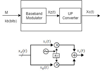
Since the up-convertor and the down-convertor processes are performed by the USRP, we can use the baseband representation of the signals.

Digital Demodulator

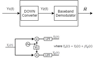
Baseband Demodulation

The baseband demodulation structure is expressed as

Digital Demodulator

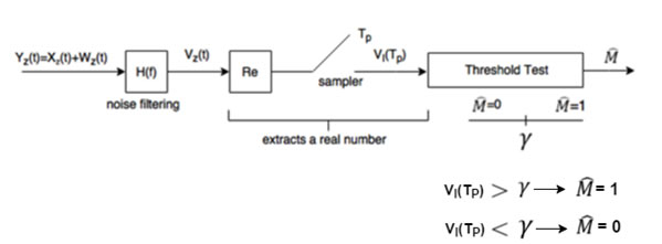
Threshold Test>

Since the distribution for two bits are Gaussian, the region between two distributions generates error messages. In order to reduce the probability of the error, which is the primary goal of designs, we set a threshold level. As seen in Figure 5, if the distribution is greater than γ, therefore the message is received as 1 or vice versa.

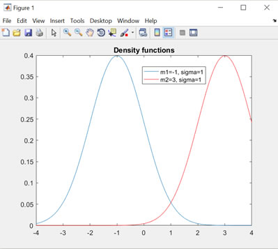
As you can see in figure 6, blue marked distribution represents $π_0 f(V_I (T_P )|M=0)$ and the red one is $π_1 f(V_I (T_P )|M=1)$, where $π_0$ and $π_1$ are the probabilities w.r.to bits 0 and 1, and f(.)s are the Gaussian distributions. The intersection is called error region. In such cases, we assume that $π_0=π_1=\frac{1}{2}$    therefore,   $γ=\frac{(m_1+m_0)}{2}$ (In Figure 6, $m_1=-1,\:\:m_2=3$).

$f(V_I (T_P )│M=0)=\frac{1}{\sqrt{2πσ_{NI}^2}} e^{-\frac{V_I-m_0}{2σ_{NI}^2}}$ and $f(V_I (T_P )│M=1)=\frac{1}{\sqrt{2πσ_{NI}^2}} e^{-\frac{V_I-m_1}{2σ_{NI}^2}}$ , where the variance is the PSD of the noise, $σ_{NI}^2=N_0 \int\limits_{-\infty}^{\infty}|H(f)|^2 df$ (depends on the noise only)

The mean values are as in the followings

The probability of error is

_B (ϵ) in terms of Q-function yields (assuming that π_0=π_1=1/2) (please see your definition of Q-function)

Matched Filter Realization: H(f)

Matched filter is the filter that is being used to minimize the probability of error $P_B (ϵ)=Q(√η)$, where P_B (ϵ) is derived previously, $P_B (ϵ)=Q((m_1-m_0)/(2σ_NI ))$ [2]

Please note that we also assume $π_0=π_1=1/2, therefore γ=(m_1+m_0)/2$.

Here, we will not derive the matched filter’s formula.

The mean values are

, and the variance

, where $∆_E (1,0)=∫_{-∞}^{+∞}|x_{z,1} (t)-x_{z,0} (t)|^2 dt$ is called Squared Euclidian Distance (SED)

Therefore, SED can also be found as

, where ρ_10 is the correlation coefficient between the waveforms $x_{z,1} (t) and x_{z,0} (t)$, then

Thus, we can rewrite the mean values are,

Finally, the probability of bit error is

BPSK: Union bound and Constellations

Since the BPSK is a single bit transmission, $x_(z,i)$ $(t)$ is defined as $(2^1=2)$

$$x_(z,i)=\Bigg\{ \genfrac{}{}{0pt}{}{(x_(z,1) (t)=\sqrt{\frac{E_B}{T_p}} , 0≤t≤T_p (for M=1)}{x_(z,0) (t)=-\sqrt{\frac{E_B}{T_p}}, $0≤t≤T_p (for M=0))} $$

The probability of bit-error is calculated for BPSK as

Linear Modulation

, where d_i is the constellation points in I-Q plane and $i=0,1,…,2^(k_b )-1$, and $u(t)$ has waveform with unit energy, then

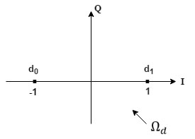
The constellation for BPSK is $Ω_d=\{d_0,d_1 \}=\{-1,1\}$ as seen in Figure 7

Performance Metrics

Probability of Error

The probability of the word error is defined as

for a single bit transmission,

Spectral Efficiency

and the $R_B$ is the bit rate (bit/sec) is defined as $R_B=\frac{k_b}{T_P}$ , where $k_b$ is the number of bits and $T_p$ is the duration of the $x_c (t)$

Transmission SNR

Energy of a signal can be found as

References

[1] Michael P. Fitz, Fundamentals of Communication Systems, pp. 12.2, 2007, McGraw-Hill

[2] ] Michael P. Fitz, Fundamentals of Communication Systems, section. 13.4.2, 2007, McGraw-Hill