Lab 2: Designing and Analyzing Frequency Modulator and Demodulator
Objective
To understand the theoretical foundations for Angle Modulation as well as Frequency Modulation (FM) and Demodulation
To implement the Simulink models for FM including a basic sinusoid and a multimedia file (music) to analyze each signal in time and frequency domains using time scope and spectrum analyzer
To examine the effects of the Additive Gaussian Channel (AWGN) in the Simulink for FM
To observe the real-time music transmission for a FM modulated music file via USRP trans-receiver
1. Theoretical Background
Amplitude modulation was the first modulation type to be considered in analog communication systems. Amplitude modulation has the obvious advantage of being simple and relatively bandwidth efficient. The disadvantages of amplitude modulation are [1]:
Since the message is embedded in the amplitude of the carrier signal, the cost, performance, and the size of the linear amplifiers are difficult to accomplish for obtaining fair performance in AM systems.
When the message goes through a quiet period in Double Side Band (DSB) or Single Side Band (SSB) systems, very small carrier signals are transmitted. The absence of the signal tends to accentuate the noise.
The passband bandwidth is small compared to the other modulation schemes, i.e. FM, cellular, Wi-Fi etc.
Angle Modulation
In the first experiment, we analyzed the effect of varying the amplitude of a sinusoidal carrier in compliance with the baseband (information) signal. A major improvement in performance in the transmission is achieved with angle modulation. In this type of modulation, the amplitude of the carrier is kept constant. Angle modulation provides the improved noise performance.
Phase Modulation, and Frequency Modulation are both the modulation techniques analyzed in angle modulation. In this second experiment, we will examine the most common modulation scheme in daily life, namely, the Frequency Modulation, or FM.
Please see the Fundamentals of Analog Communications section as discussed in the first experiment as a reference.
Frequency Modulation
The angle modulated signal described in time domain:
$s(t)=A_c cos[2πf_c t+θ(t)]=Re\{Aexp(jϕ(t)\}$ where $A_c$ is the amplitude, then
The instantaneous phase is: $$ϕ_i=2πf_c t+θ(t) $$
The instantaneous frequency of the modulated signal is:
$ f_i (t)=\frac{1}{2π} \frac{d}{dt} [2πf_c t+ θ(t)]=f_c+\frac{1}{2π} \frac{d[θ(t)]}{dt}$ where $\frac{d[θ(t)]}{dt}$ is called phase deviation.
The phase deviation of the carrier $ϕ(t)$ is related to the baseband message $m(t)$. Then,
$\frac{d[θ(t)]}{dt} = K_f m(t), K_f: frequency \ deviation \ constant$
$$ϕ(t) = K_f ∫_{-∞}^t m(λ)dλ$$
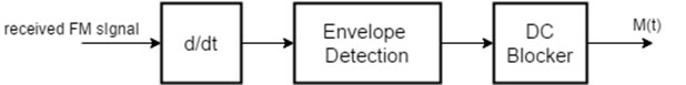
Finally, the frequency modulated signal is expressed as in time domain:
The differentiated signal is both amplitude and frequency modulated, the envelope $ A_c [2πf_c+K_f m(t)] $ is linearly related to message signal (amplitude component) and $ sin\Big(2πf_c t+2πK_f ∫_{-∞}^t m(λ)dλ\Big)$ is high frequency component. Therefore, m(t) can be recovered by an envelope detection of $ ds(t)/dt $.
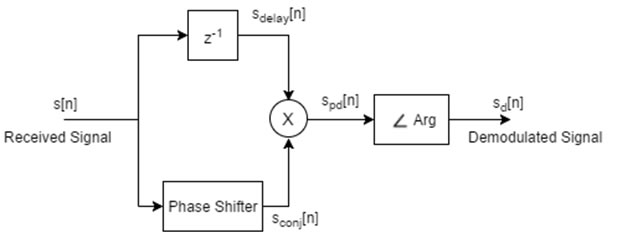
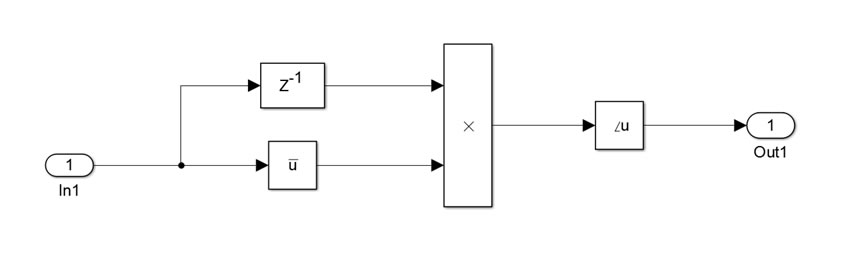
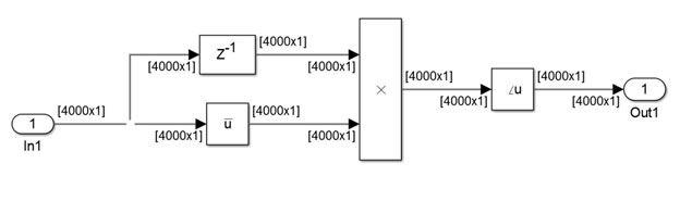
Non-Coherent FM Demodulation
It is also called as Complex Delay Line Frequency Demodulator derived using the blocks as shown
The complex received FM signal have both real and imaginary components. This signal has the form:
$$ s(t)=A_c e^{j(2πf_c t+θ_FM (t))} $$
The complex received signal is the input to two blocks. The Phase Shifter block is used to take the conjugate of the signal to change the phase, and the Delay block, z^(-1) adds time delay to the signal to retard it.
During the USRP experiment in FM, we will use the non-coherent demodulator structure.
For more information, refer to [3].
PLL Demodulation
The PLL demodulates the FM signal using feedback force a Voltage-Controlled-Oscillator (VCO) to remain in phase with the carrier of the incoming signal. The message is recovered as the control input of the VCO [4]. In the simulation experiment (section-2), we used the VCO to demodulate the information signal to make life easier.
2 Building Simulink Model of Frequency Modulation and Demodulation
The frequency modulator and demodulator structures are as explained below. In the first model, you are provided a FM structure that is very similar to the theoretical background of this experiment. In the second model, you will observe the frequency variations with respect to the input signal’s waveform. In this case, you will use the modulator and demodulator blocks provided by Simulink.
Model-1
Frequency Modulation
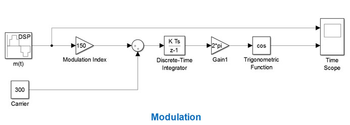
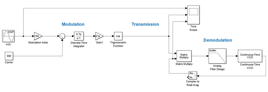
The Simulink model for FM modulator is:
Figure 1: Block Diagrams for the FM Modulator
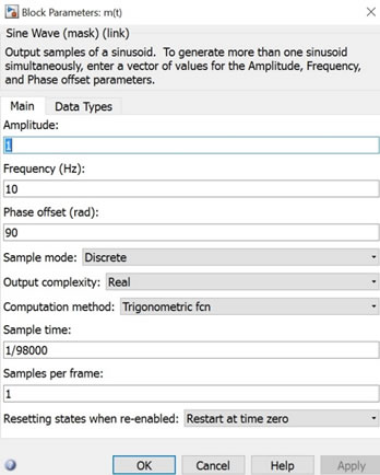
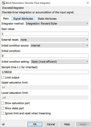
The blocks’ parameters are as described below:
Figure 2: Blocks’ Parameters for FM Modulator
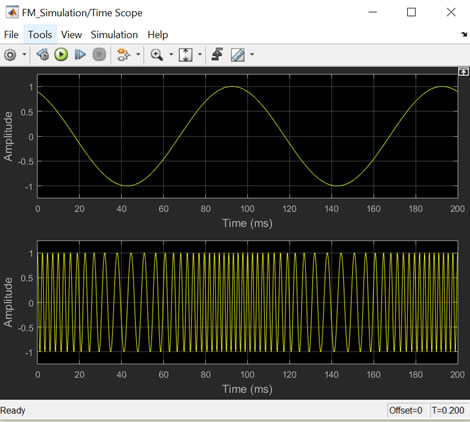
Adjust the simulation time about 0.2 sec to observe the waveforms precisely.
The result in time scope will be:
Figure 3: Time Scope
Frequency Modulator and Demodulator
The Simulink model of the complete FM modulator and demodulator is shown next:
Figure 4: FM Modulator and Demodulator
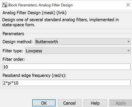
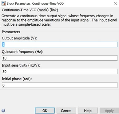
You need the modify the filter and the VCO parameters as shown in the screenshots:
Figure 5:Block Parameters
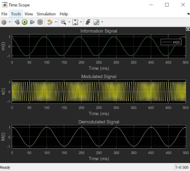
Run your simulation and observe the signals in the time scope:
Figure 6: Time Scope for Model-1
As you can see, the FM modulated sinusoid is recovered in demodulation.
Model-2
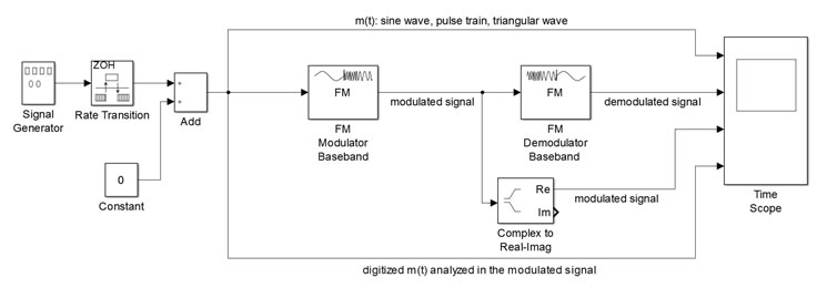
In model-1, you have already learnt the theoretical foundations for FM. In the second model, instead of using complex modulator and demodulator structure, we will implement an FM system using direct modulator and demodulator blocks defined in Simulink. The input, in this case, has three different forms: sine wave, rectangular pulse train and triangular waves. Therefore, we will be able to observe the frequency variations using variety of inputs. The model-2 is expressed as:
Figure 7: FM Model-2
The signal generator block is simply an analog input. In order to use this block as an input of the FM Modulator, we need to digitalize it. The rate transition block (zero-order-hold, or ZOH) will sample the analog information by the sampling period (please see the Review Manual for the sampling process). in this case, $T_S$ equals to $1/100e3$.
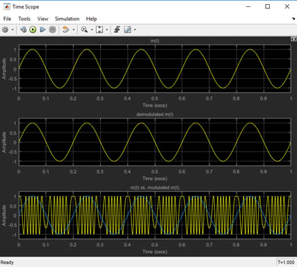
Take the input signal’s frequency as 5 Hz (use sine wave), and set the frequency deviation for the modulator and demodulator as 100 Hz, respectively. Also, adjust the time scope as three vertical layouts in order to analyze the $m(t)$ vs. the modulated $m(t)$.
The resulting time scope will be:
Figure 8: Time Scope for Model-2
Similarly, the $m(t)$ is fully recovered.
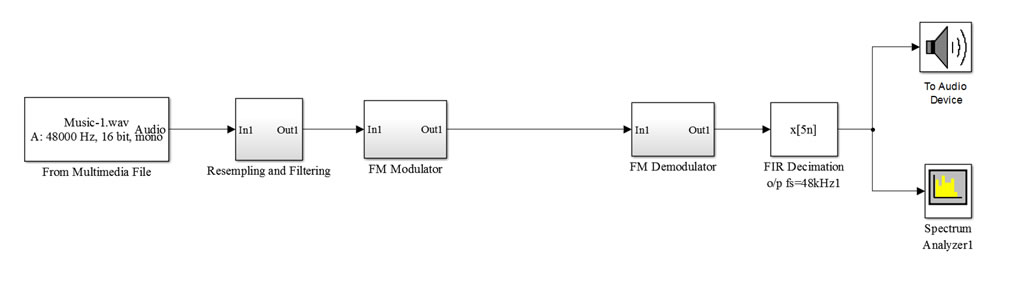
3. Building Simulink Model for Music Transmission using FM Modulator and Demodulator (Baseband)
Here, we will implement the FM modulator and demodulator using a music file as a source. In this case, since the source is a multimedia file rather than a pure sine wave, we need DSP processing, which is resampling and filtering. You will not be kept responsible for DSP processes. However, you can find them very useful when comprehending sampling rate, rate conversion, Finite Impulse Response (FIR), decimation and interpolation etc. You can also check the following resource:
Chapter 3, Multiresolution Signal Decomposition, Ali N Akansu, Haddat.
The model is shown below.
Figure 9: Simulink Model for Music Transmission using FM Modulator and Demodulator
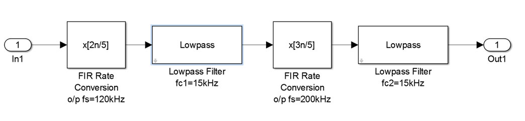
Figure 10: Resampling and Filtering Block
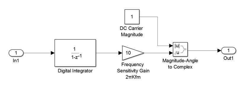
Figure 11: FM Modulator Block
Figure 12:Non-Coherent FM Demodulator Block
4. Transmitting and Receiving a Multimedia File using FM via USRP
Now, we will go a further step to transmit a music file, and then receive it via USRP hardware. In this case the transmission is real time, therefore unlike the simulations, you will observe the transmission through the air as well as the noise.
The model is expressed as:
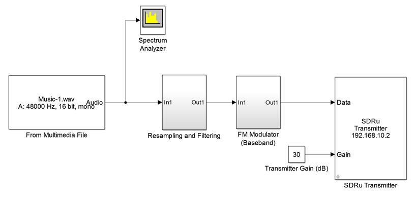
Transmitter (TX)
Figure 13: Simulink® Design of a Multimedia File Transmission Using FM Modulation
Resampling and Filtering blocks are the same as the music simulation as well as the baseband modulator.
Plot $|M(f)|$, and find the energy of $m(t) (f_m=100 Hz)$
Find the bandwidth of the FM signal $(f_m=100 Hz,K_f=1000)$
6. Lab Tasks
Perform the following tasks:
Build the model-1 (figure 1). Explain the modulation part as in figure 1 by describing each step by $m(t),K_f$, etc.
Complete the model 1 by adding demodulator as in figure 4. Then, explain how modulation and demodulation take place.
Add an Additive White Gaussian Noise (AWGN) channel into the 1-a. Play with the variance values. What happens to your modulated signal when you increase the power of the noisy channel?
Build the model-2 as in figure 7. .
Explain how modulation and demodulation take place by commenting time scope and spectrum analyzers.
We would like to have a periodic pulse train in this case, therefore we need to modify the source by changing its magnitude and shifting on the vertical axis. The following steps should be performed in the beginning:
Switch the signal generator waveform to square wave with amplitude of 0.5
Connect an Add block to the source and add a constant value of 0.5
Run your simulation, then explain the frequency variations with respect to the input signal. Finally, perform the steps in 2).
Open the FM_Music_Simulation.slx file on your computer. Explain steps in the FM music simulation file. Then, proceed the steps in task-2.
Open, and then run AM_Music_Simulation file on your computer. Compare the quality for both AM and FM. Which one do you think is better?
Steps: USRP
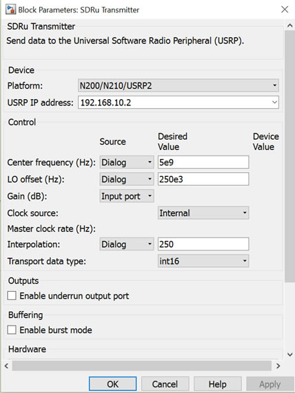
Ask your instructor to open, and then run the TX_FM_Music.slx file. Check the block diagrams for the transmitter (You will find no difference than the music simulation, but the transmitter). Take note the transmitter central frequency.
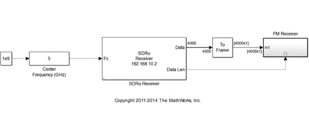
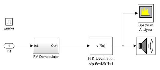
Open the RX_FM_Music.slx file in your computer. Set the central frequency the same as the transmitter, and then run the file. Observe the real-time transmission through the air.
7. Lab Report Instructions
Please see the instructions in the course web site.
8. References
[1] M. P. Fitz, Fundamentals of Communications Systems, pp. 7.1-7.7, 2007, McGraw-Hill
[2] Hwei P. Hsu, Schaum’s Outlines of Theory and Problems of Signals and Systems, pp.1-5, 1995, McGraw-Hill
[3] Robert W. Stewart, Kenneth W. Barlee, Dale S.W. Atkinson, and Louise H. Crockett, Software Defined Radio using MATLAB & Simulink and the RTL-SDR, pp. 355-358 and figure 9.17, Strathclyde Academic Media, 2015
[6] Robert W. Stewart, Kenneth W. Barlee, Dale S.W. Atkinson, and Louise H. Crockett, Software Defined Radio using MATLAB & Simulink and the RTL-SDR, pp. 370-375, Strathclyde Academic Media, 2015
[9] Robert W. Stewart, Kenneth W. Barlee, Dale S.W. Atkinson, and Louise H. Crockett, Software Defined Radio using MATLAB & Simulink and the RTL-SDR, pp. 371, Strathclyde Academic Media, 2015