Lab 4: QPSK modulation
Objective
In this lab, you will observe the Quadrature Phase Shift Keying (QPSK) modulation and demodulation building Simulink simulation. Then, the second stage will be the implementation of QPSK using USRP Hardware.
Prelab
- Draw the constellation diagram for QPSK. Which bit does each point represent?
- What is the difference between Binary code and Gray code? Which one is better?
- What is the trade-off of using QPSK over BPSK?
Building Simulink Model of QPSK Modulator and Demodulator
- Standard QPSK Simulation
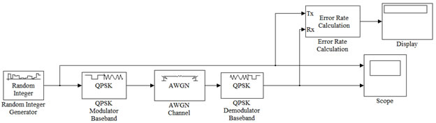
- Build the Simulink model shown in Figure 1.
- Double-click on the Random Integer Generator and adjust the set size to a proper value (Remember that the input to the QPSK modulator should be either 0, 1, 2, or 3).
- In the Random Integer Generator block, set the Sample Time to 1e-6 (i.e. 1 µs) and the Samples per frame parameter to 1024.
- In the AWGN block, set the Symbol period parameter to 1e-6 (i.e. 1 µs) and the Number of bits per symbol parameter to 2 (since QPSK uses 2 bits per symbol).
- For the Error Rate Calculation block, set the Output data field to “port” so you can connect the Display block.
- The Display Block will show you three values. The first value is the BER, the second value is the number of incorrect bits, and the third value is the total number of bits received.
- Set the simulation time to 10 seconds.
- In both QPSK Modulator and Demodulator blocks, set the Constellation ordering to Gray. Take a note of the constellation points.
- In this experiment, you will adjust the value of the in the AWGN block, starting from 3, incrementing by 1 every step, and ending at 15, and observe the error rate displayed in the Display block. Make a table recording the value of and the corresponding BER.
- Plot BER vs. and compare with the theoretical values. Comment on the results.
- Repeat for Binary Constellation ordering in both QPSK modulator and demodulator blocks and comment on the results.
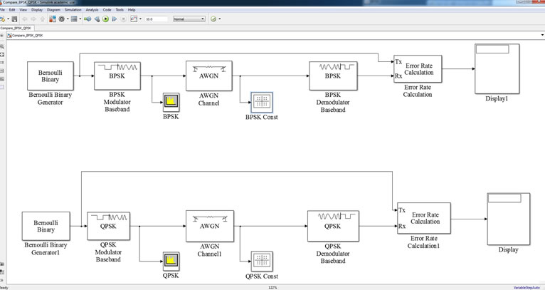
- Comparing QPSK and BPSK
- Build the Simulink model shown in Figure 2.
- Double click on the Bernoulli generator for the BPSK part. Set the sample time to 1e-6 and the Samples per frame to 1024.
- Double click on the Bernoulli generator for the QPSK part. Set the sample time to 0.5e-6 and the Samples per frame to 1024.
- For the QPSK Modulator and Demodulator blocks, use Gray Constellation ordering.
- Choose the same value of SNR for both AWGN blocks
- Set the simulation time to 10 seconds.
- Run the simulation and observe the bit error rate and the number of transmitted samples from the Display block for both schemes, and observe the used bandwidth for both schemes from the spectrum analyzer block. Explain your observations.
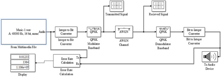
- A Music File Transmission with QPSK
- The music file that you will use (named Music-1.wav) is located on the Desktop.
- The music file length is 62 second, so set the Simulation Time to 62 seconds.
- In this experiment, you will adjust the value of SNR in the AWGN block and observe the quality of the music. Choose at least three values of SNR (high, mid, low) and comment on the quality of the music.
The Simulink model of QPSK modulator and demodulator is shown below
In this experiment, you will learn about the trade-off of using QPSK over BPSK.
The following model will be used to simulate a music file transmission using QPSK modulation with AWGN channel. You will observe both constellations in the transmitter and the receiver sides and the Bit Error Rate.
QPSK Modulator and Demodulator Using USRP Hardware
In this part, you will learn that for real-time transmission, it is not enough just to have a demodulator block to regenerate the transmitted message. There are other issues that need to be dealt with such as Phase errors and Synchronization.
- Standard System
- Double-click the file named QPSK1.mat in the MATLAB window. This will load the parameters that are used in the receiver block diagram.
- Open the file named QPSK1.slx. This model represents the receiver side. The transmitter side is already running.
- Run the model and observe the output in the MATLAB window. Take a snap shot of the constellation diagrams at every stage and comment on the plots.
- Phase Errors Issues
- Open the file named QPSK_Phase_Error.slx. This file is the same as the previous one except that the phase cancellation block is removed.
- Run the model and observe the output in the MATLAB window. Take a snap shot of the constellation diagrams at every stage and compare with the plots from the previous section.
- Time Synchronization Issues
- Open the file named QPSK_Time_Sync.slx. This file is the same as the file from the first section except that the Time Synchronization block is removed.
- Run the model and observe the output in the MATLAB window. Take a snap shot of the constellation diagrams at every stage and compare with the plots from the first section.