Lab 1: Amplitude Modulator and Demodulator
Objective
- To understand the theoretical foundations of Analog Communications as well as of Double-Side-Band Amplitude Modulation and Demodulation (DSB-AM)
- To design the Simulink model of the DSB-AM to analyze each signal in time and frequency domains using time scope and spectrum analyzer
- To examine the effects of the Additive Gaussian Channel (AWGN) in the Simulink Model of DSB-AM
- To observe the real-time music transmission for DSB-AM modulated signal via USRP trans-receiver
Theoretical Background
- Review of Signals & Systems, Probability and Noise and Starters’ Guide
- Fundamentals of Analog Communications
- Size of the antenna reduces when a signal is modulated by a larger frequency of a carrier.
- Using modulation to transmit the signal through space to long distances. Therefore, Wireless Communication techniques has raised our standards considerably.
- Modulation allows us to transmit multiple signals in the same medium (i.e. Frequency Division Multiplexing, FDMA)
- Amplitude Modulation and Demodulation
In order to understand the theory along with the experiments behind this course, the review sections were prepared. It is highly recommended that the Review and the Starters’ Guide are understood. Please see the instructor for any further information.
As a reminder, Review of Signals & Systems, Probability and Noise is valid for all experiments.
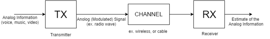
Analog Communication is an information transmitting mechanism, i.e. music, voice, and video using broadcast radio, walkie-talkies, or cellular radio, and broadcast television. The significant invention made by Marconi in 1895 was a radio. Later, the foundation of Trans-Atlantic Communication Systems had been taken place. Although digital communications systems are much more efficient, cost-saving, more reliable, some communication systems are still analog.
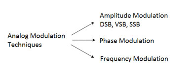
Analog communication techniques can be summarized as
Advantages of modulation:
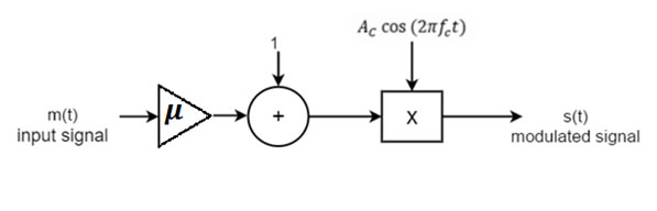
Let $ω_c = 2πf_c$ be the carrier frequency in radians per second where where $fc >> W$. Then the amplitude modulated signal $s(t)$ can be expressed [1] (H. Taub, 2008, p. section 3.3) as
$$s(t)=A_C \Big[1+μm(t)\Big]cos(2πf_c t)$$ $$s(t)=A_C cos(2πf_c t)+A_c μm(t)cos(2πf_c t)$$, where $u$ is the modulation index defined in $-1<μ<1$
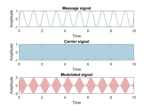
As an example, the following figure shows the Amplitude Modulation with $m(t)=sin(2πt),\:A_C=1,\:μ=0.9, \:and \:f_c=10 Hz$,
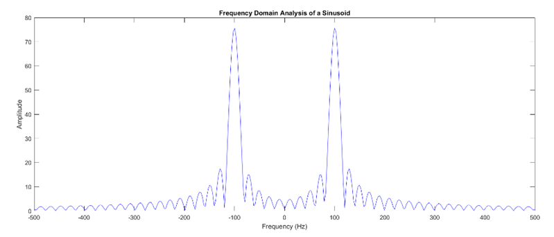
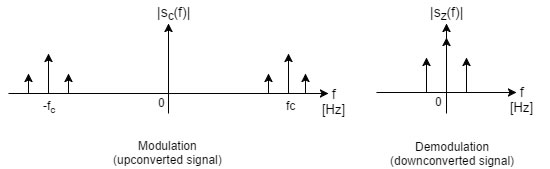
Recall: Modulation Property
$m(t)$ is multiplied by $cos(2πf_c t)$; $$m(t)∙cos(2πf_c t)⟺\frac{1}{2}\Big[M(f-f_c )+M(f+f_c )\Big], \:where\: f\: is\: the\: freqency\: of\: m(t)$$
In general, the AM modulation is summarized as:
In case of carrier, which could be used sine or cosine wave. Practically, there is no difference except -90-degree phase shift.
Remark:
Any signal is summed by a constant value means that this signal is raised by the same constant value with respect to the vertical axis in time domain. In frequency domain, the constant value is represented by an impulse at $f=0\: Hz$.
Demodulation
For AM demodulation, we will examine the Square-Law and Envelope Detector techniques.
Demodulation by Squaring
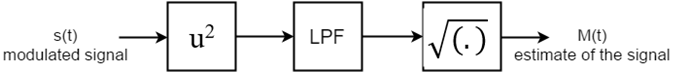
The high frequency is removed after filtering,
$$=\frac{1}{2} \Big(1+μm(t)\Big)^2, \:\:then$$ $$M(t)=\frac{1}{4}\Big(1+μm(t)\Big) $$Synchronous Demodulator
The block diagram of synchronous demodulator is as shown
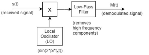
In order for the low-pass to detect the information envelope, the frequency of the carrier must be as high as possible. However, as you can imagine the noise from the nature (i.e. white noise) cannot be filtered/removed perfectly in such analog transmissions (AM, or FM).
$$s(t)=sin(2πf_c t)+\frac{m(t)}{2} sin(2πf_c t-2πf_m t)-\frac{m(t)}{2} sin(2πf_c t+2πf_m t)$$After the multiplication of $s(t)×sin(2πf_c t)$
$$ =-\frac{m(t)}{2} sin(2πf_m t)-\frac{1}{2} sin(2πf_c t)-\frac{m(t)}{2} (4πf_c t-2πf_m t)+\frac{m(t)}{4} sin(2πf_c t+2πf_m t) $$Then, the low-pass filter removes the higher frequency components, so we can recover m(t).
2. Building Simulink Model of Amplitude Modulator and Demodulator
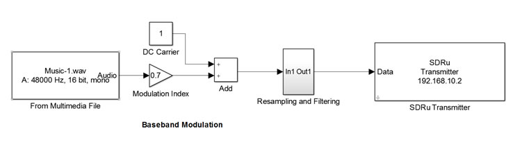
Modulation
The Simulink design of an Amplitude modulator is in the following [2] (M. Boulmalf, 2010)
Parameters:
- Double click on the signal generator, and then set the frequency as 1 kHz with a waveform of sine
- Adjust the carrier sine wave’s frequency as 20 kHz
- Set the simulation time such as 0.01 to observe the signals clearly
- Run your simulation
- In order to observe the spectrum analyzer, please increase the simulation time to 1 or 2 seconds.
As it is clearly seen that the AM model is exactly based upon the mathematical foundation provided in the theoretical section. The message signal is multiplied by the modulation index, then it is added a DC carrier, finally is multiplied with a sinusoidal carrier signal in order to transmit the AM modulated signal.
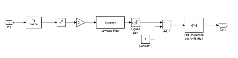
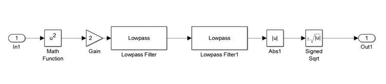
Demodulation (Square-Law Demodulator)
Apply the similar procedure. You will have the demodulation structure as shown in the following figure:
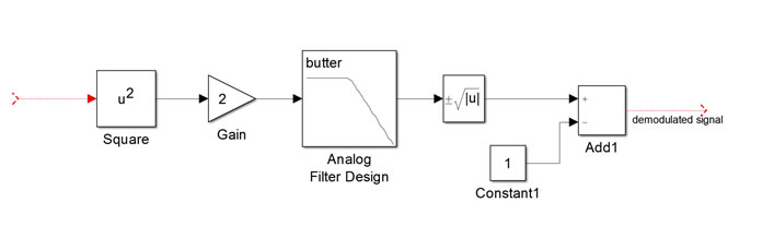
- Specify the band edge frequency as 2*pi*X
Connect your modulation and demodulation models as shown.
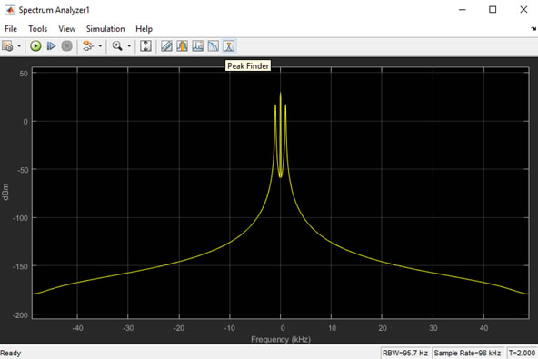
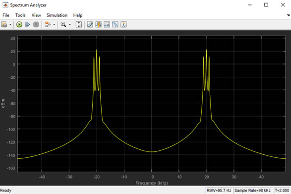
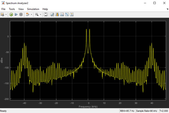
Run your model, you will then observe the following
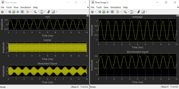
Simulation time is chosen to be 2 secs for the spectrum analyzers.
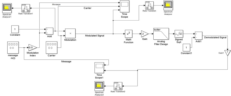
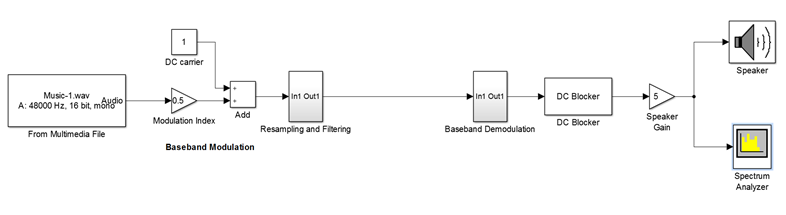
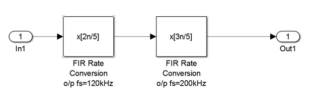
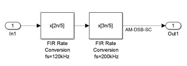
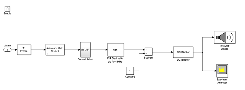
3. Building Simulink Model of the Music Transmission Using DSB-AM Modulator and Demodulator (Baseband)
Here, we will implement the DSB-AM baseband modulator and demodulator using a music file as a source. In this case, since the source is a multimedia file rather than a pure sine wave, we need the DSP process, which is the resampling and filtering. You will not be kept responsible for DSP processes. However, you can find them very useful when comprehending sampling rate, rate conversion, Finite Impulse Response (FIR), decimation and interpolation etc. You can also check the following resource:
Chapter 3, Multiresolution Signal Decomposition, Ali N Akansu, Haddat.
The model is shown below.
Transmitting and Receiving a Multimedia File using DSB-AM via USRP
Now, we will go one further step to transmit a music file, and then receive it via USRP hardware. In this case the transmission is real time, therefore unlike the simulations, you will observe the noise through the air.
The model is expressed as
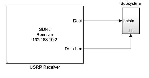
Transmitter (TX)
Receiver (RX)
5. Prelab Instructions
- Starters Guide and Signals and Systems Review Manuals
- Answer the following questions:
- Plot the magnitude of the following waves in frequency domain by hand
- $1 + sin(4πt)$
- $A_C[1 + sin(4πt)] cos(80πt)$, where $A_c$ is a positive number
- The message signal $m(t) = sin(4πt)$
- Plot $|M(f)|$ by hand
- If this message is DSB-AM modulated on a carrier $cos(80πt)$, find the corresponding passband modulated signal $s_c (t)$ and plot $|S_c (F)|$ by hand
- The received signal $s_c (t)$ is the input of the demodulator as described below:
- Find the $y(t)$, and then compare it with $m(t)$. Did you recover the signal? Comment your result.
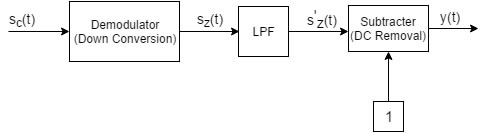
The passband received signal after the demodulation is converted to baseband. This process is simply:
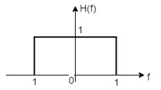
The LPF has the following specifications:
There are two additional supplements, Simulink and USRP Starters Guide and Review of Signals and Systems, were prepared and added to the course web site. You will find them very useful while answering prelab questions and comprehending lab tasks.
6. Lab Tasks
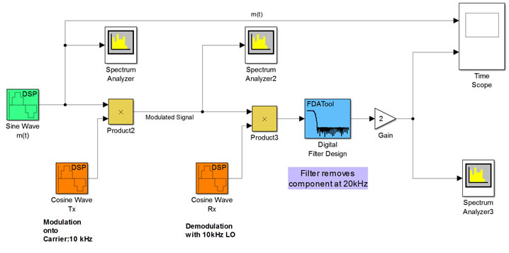
- [Synchronous Detector]
- m(t) with frequency of 1kHz and sample time:1/100kHz
- carrier: 10kHz, phase:$π/2$ and sample time: 1/100kHz
- Local Oscillator (LO): same as carrier.
- Filter: LowPass, Fs:100kHz, Fpass:6 and Fstop:12
- Set up the simulation time as 50k/100k
- Run your model
- Observe the 3 spectrum analyzers, then explain the waveforms from the frequency point of view (Hint: remember modulation property). Comment your result.
- Change the simulation time to 500/100k (to clearly see the sine wave). Compare signals in the time scope? Did you recover m(t)? Is there any delay between two signals? If yes, explain, why?
- Build the Simulink model of AM modulator and demodulator (Figure-7) explained in this manual. You must determine the analog filter’s passband edge frequency. Then, explain the theoretical side of the blocks. Use the notation as μ:modulation index, $m(t), h(t)$, etc.
- As the nature of transmission, the message can be distorted in different levels by the noise, which may occupy between specific frequencies, i.e. colored noise, or all frequencies, i.e. White Gaussian Noise (WGN). The following block is called “Additive White Gaussian Noise”.
- Set the modulation index μ as -10, -5, -0.9, -0.1, 0.5, 0.9, 5, 10 respectively.
- What happens to the modulated signal’s waveform for each case?
- In which values, the demodulation can be performed correctly? Why?
- Find the AM_Music_Simulation.slx file on your computer, then run the model. Similarly, answer the questions in task-2 based on this model.
- Steps: USRP
- Ask your instructor to open, and then run the TX_AM_Music.slx file. Check the block diagrams for the transmitter (You will find no difference than the music simulation, but the transmitter). Take note the transmitter central frequency.
- Open the RX_AM_Music.slx file in your computer. Set the central frequency same as the transmitter, and then run the file. Observe the real-time transmission through the air.
- Self-Study:
Type the following code in the command window [4]:
>> dspenvdet - Run your simulation to observe the waveform in time domain
- Click on dspEnvelopeDetector.m, then run the m-file. Observe the Matlab figures in both envelope detection techniques
Build the model given below [3], and then set up the block parameters as
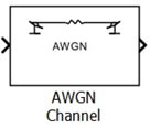
Connect the AWGN channel. Set the variance from mask as 0.01, 0.05, 0.1 and 0.5 respectively. What do you observe in each case? Comment your result
This code will open the Simulink Model of DSB-AM modulator and demodulator techniques based on Envelope Detector by Squaring and Hilbert Transform.
7. Lab Report Instructions
Check out the template in the course web site.
8. References
[1] H. Taub, D. L. (2008). Principles of Communication Systems (3rd ed.). McGraw Hill.
[2] M. Boulmalf, Y. S. (2010). Tearching Digital and Anolog Modulation to Undergraduate Information and Technologhy Students Using Matlab and Simulink. IEEE.
[3] Simulink model of Perfect Modulation and Demodulation, Software Defined Radio using MATLAB & Simulink and the RTL-SDR, Strathclyde Academic Media, 2015
[4] The Mathworks Inc ®, Envelope Detection,