Lab 2: Power Transformer Open and Short Circuit Tests
Objectives
- To conduct standard open and short circuit tests in order to find the parameters of the equivalent circuit of a transformer.
- Evaluate the regulation and efficiency of the transformer at a given load.
- Check the excitation characteristics of the transformer.
Equipment
- One Power Quality meter from the stockroom.
- Two scope leads from the stockroom.
- One McLean Engineering Transformer EP-Trio with .1 MOHM-1 microfarad integrator and two 25 Watt 1 Ohm resistors built into back.
- 3-phase AC Variac.
- One four-winding single phase transformer. (Model # T-1000)
- One oscilloscope.
References
- A. Fitzgerald, C. Kinsley, Jr., S. Umans, Electric Machinery, Ch. 1,
6th Edition, McGraw-Hill Inc., 2005.
- P.C SEN, Principles of Electric Machines and Power Electronics, 3rd Edition, John Wiley, 2013
Background
A power transformer is usually employed for the purpose of converting power, at a fixed frequency, from one voltage to another. If it is used for converting power from a high voltage to a low voltage, it is called a step-down transformer. The conversion efficiency of a power transformer is extremely high and almost all of the input power is supplied as output power at the secondary winding.
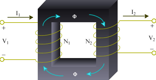
Figure 3.1: Ideal transformer
Consider a magnetic core as shown in figure 3.1, carrying primary and secondary windings having N1 and N2 turns, respectively. When a sinusoidal voltage is applied to the primary winding, a flux Φ will exist in the core which links both the primary and secondary windings, inducing the RMS voltages
The transformer is said to have a transformation ratio
Prelab
Determine how to connect the meters into the circuits:
- Figure 3.4 (Open Circuit Test) to measure the voltage ( V1), current ( Ip), and power ( Woc) of the transformer.
- Figure 3.5 (Short Circuit Test) to measure the voltage ( Vsc), current ( Isc ), and power ( Wsc) of the transformer.
Show connections for each circuit with (a) regular Wattmeter (4 terminals) (b) Power Quality Meter (Fluke 43B)
Equivalent Circuit
The transformer may be represented by the equivalent circuit shown in figure 3.2. The parameters may be referred to either the primary or the secondary side. The series resistances R1 and R2 represent the copper loss in the resistance of the two windings. The series reactances X1 and X2 are leakage inductances and account for the fact that some of the flux established by one of the windings does not fully couple the other winding. These reactances would be zero if there were perfect coupling between the two transformer windings.
Figure 3.2: Equivalent circuit of a transformer.
The shunt resistance Rp accounts for the core losses (due to hysteresis and eddy currents) of the transformer. The shunt inductance Xp is representative of the inductances of the two windings and would be infinite in an ideal transformer if the number of turns of the two windings were to be infinite.
A knowledge of the equivalent circuit parameters permits the calculation of transformer efficiency and of voltage regulation without the need to conduct actual load tests. But experimental data must first be obtained in order to determine those parameters.
It will be confirmed at the conclusion of the first two parts of this experiment that the impedances of the series branch of the transformer equivalent circuit are substantially smaller than the impedances of the parallel branch. Because of this large discrepancy in the magnitudes of the elements we can redraw the equivalent circuit shown in figure 3.2 into that shown in figure 3.3. The errors introduced into calculations using figure 3.3 in place of figure 3.2 are quite insignificant. Furthermore, the large difference in the magnitudes of the transformer parameters allows for the determination of the elements in the series branch using one set of measurements and the elements in the parallel branch using another set of measurements.
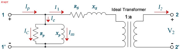
Figure 3.3: Simplified equivalent circuit of a transformer.
Open Circuit Test
The open circuit test is used to determine the values of the shunt branch of the equivalent circuit Rp and Xp . We can see from figure 3.3 that with the secondary winding left open, the only part of the equivalent circuit that affects our measurement is the parallel branch. The impedance of the parallel branch is usually very high but appears lower when referred to the low voltage side. This test is therefore performed on the low voltage side of the transformer terminals 1 − 1' in figure 3.3) to increase the current drawn by the parallel branch to a readily measurable level. Besides, the rated voltage on the low voltage side is lower and therefore more manageable.
T-1000 transformer has four windings. Create a 1:2 ratio step up transformer by connecting the two primary windings in series and the two secondary windings in series.
This transformer will also be used in the next part of the experiment, so leave the connections intact when the present part is finished.
This transformer is rated at 1.0 KVA. The rated current is 1000 VA/240 V = 4.16A on the 240 V side and 1000 VA/120 V = 8.32A on the 120 V side.
Figure 3.4: Circuit for open circuit test.
Instructions
- Connect the circuit as shown in figure 3.4. Make sure that the low voltage side of the transformer corresponds to the left side of the connection diagram. A low power factor wattmeter should be used.
- Connect the Power Quality Meter to the left side (primary) of the transformer. If a low Power Factor Wattmeter is used, it should be connected also to primary and DVM’s connected to allow measurement of phase voltage (V1) and primary current (IP)
- Connect the power supply from the bench panel to the INPUT of the three-phase variac and connect the OUTPUT of the variac to the circuit.
- Vary the input voltage starting at 0 V in 20 V increments to go up to 120 V. At each step change, record Ip , W0 and V1 in table 3.1.
- Turn off the variac.
Report
- Complete table 3.1
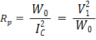
- Compute the parameters Rp and Xp at the rated voltage by using
- Find the value s of Rp and Xp as referred to the high voltage side.
- Plot the no-load current Ip , magnetizing current Im , core loss W0 and no-load power factor cos Φ , against the applied voltage V1 on the same graph paper.
| Table 3.1: Data for open circuit test. | |||||
| V1 Volts |
Ip Amps |
W0 Watts |
Ic = W0 / V1 Amps |
Amps |
cosφ = W0 / V1 Ip |
| 20 40 60 80 100 120 |
|
|
|
|
|
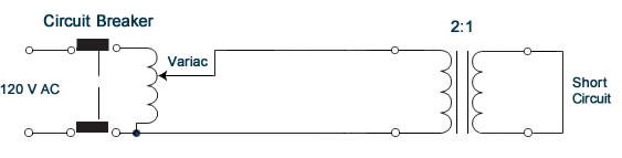
Figure 3.5: Circuit for short circuit test.

These parameters are referred to the low voltage side.
Short Circuit Test
The short circuit test is used to determine the values Rs and Xs of the series branch of the equivalent circuit. These impedances are usually very low, but appear higher in value when referred to the high voltage side. This test is consequently performed on high voltage side of the transformer (terminals 2 − 2ʹ in figure 3.3) in order to keep the current drawn by these impedances at a manageable level.
| Table 3.2: Data for the short circuit test. | ||
| Is Amps |
Vs Volts |
Ws Watts |
| 4.0 3.5 3.0 2.5 2.0 1.5 1.0 0.5 |
|
|
Instructions
- Using the 2:1 ratio transformer of the previous part connect the circuit as shown in figure 3.5. Make sure that the high voltage side of the transformer corresponds to the left side (primary) of the connection diagram. Use the voltage terminals ± and 150 V of the standard AC wattmeter, if used.
- Make sure that the variac is turned all the way down before starting this experiment. Turn on the variac.
- Turn the variac up slowly until the current Is (consult figure 3.5) is at the rated value (about 4 amps). Record Is, Vs and Ws in table 3.2.
- Repeat the previous step by reducing the current Is in 0.5 A and record all values in table 3.2.
- Turn off the variac.
Report
- Plot the copper losses Ws against the current Is.
- Compute the equivalent circuit parameter Rs and Xs at the rated high voltage winding current by first calculating
- Calculate the values of Rs and Xs referred to low voltage side.
- Now that we have all the parameters for the transformer equivalent circuit, compute the voltage regulation at the rated power and at a lagging power factor of 0.8.
- Calculate the per unit efficiency at the rated power and at a lagging power factor of 0.8.


The above results can then be used to find
These parameters are referred to the high voltage side.
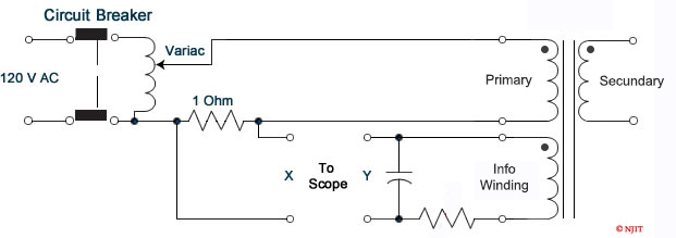
Figure 3.6: Circuit for obtaining transformer excitation characteristics
Excitation Characteristics
Instructions
- Return the T-1000 transformer and get a McLean Engineering Transformer from the cabinet.
- Connect the circuit as shown in figure 3.6.
- Apply 20 volts (peak to peak) to the primary side of the transformer.
Display and record the voltage and phase shift polarity waveform of both primary and secondary sides on a two channel oscilloscope. - Display the voltage across the 1 Ω resistor (which represents the excitation current of the primary winding) and the voltage of the secondary side on an oscilloscope and record their waveforms. Notice the non-sinusoidal of the excitation current waveform and the phase shift relative to the secondary voltage.
- Disconnect the secondary side scope leads from transformer.
- Use the optically coupled usb cable to connect your meter to the computer. Start the Flukeview software on the computer and make certain that it connects with your meter. If not, look at the device manager to determine the port that it is connected to and then choose that port for the Flukeview software.
- Vary the applied voltage and observe the change in the non-sinusoidal nature of the excitation current. At 20 Vrms and at 120 Vrms examine the voltage and current harmonics. Determine THD and the principle one or two harmonic numbers. Use the Fluxview software to capture this waveform for your report. It is best to capture the data into an excel spread sheet so that you can manipulate the plot for best viewing.
- Apply the excitation current to channel I of the oscilloscope. Display the voltage across the capacitor of the R-C passive integrator available on the back of the transformer on channel II of the oscilloscope. The purpose of the integrator is to integrate the voltage in order to get the flux since e = N (dΦ/dt).
- Press the X-Y button on the oscilloscope to see the hysteresis loop.
- Increase the voltage applied to the primary winding and record the change in the shape of the hysteresis loop.
Report
Show the captured waveforms and THD information.
Discussion Questions
- Calculate the value of the maximum efficiency of the Hampden Transformer and determine the current at which it occurs.
- Explain the differences in the harmonic contents of the current at 20 V and 120 V. Why are some harmonics missing from the current waveform at 120V?
- Using the laboratory data, determine percent efficiency of the Hampden Transformer at half rated power and 0.8 lagging power factor.